Half-Band Filters, a Workhorse of Decimation Filters
- Introduction
- What is a Half-Band Filter?
- Designing a Half-Band FIR filter with pyFDA
- Designing Perfect-Zero Half-Band Filters with a Trick
- Half-Band Filter Design with NumPy
- Using Half-Band Filters in Decimating Filters
- Conclusion
- References
Introduction
This is the 5th part in my ongoing series about converting the single-bit data stream of a PDM microphone into standard PCM samples. Check out the the References section below for the other installments.
Earlier, I already discussed how to design generic FIR filters. In this installment, I impose some restrictions on the filter, which makes them less generic, but we get something very valuable in return: an almost 50% reduction in the number of multiplications!
The plots below were all generated with Numeric Python scripts. You can find the code here.
What is a Half-Band Filter?
According to Wikipedia, “a half-band filter is a low-pass filter that reduces the maximum bandwidth of sampled data by a factor of 2 (one octave).”
When we start out with a sample rate Fs, the bandwidth of that signal goes from 0 to Fs/2. A half-band filter is used to reduce the bandwidth to Fs/4.
By itself, this is nothing special: you could do that with a generic FIR filter.
But something very interesting happens when you make the magnitude frequency response of the filter symmetric along both the frequency axis and the magnitude response axis.

In this case, the coefficient of every other filter tap, except for the center coefficient, becomes zero. For linear phase filters, coefficients will be symmetric around the center tap as well, with the center coefficient having a value of 0.5.
Here’s an example of some random half-band filter:

You can see how everything in the linear(!) magnitude response graph is perfectly symmetric around the point at (0.25, 0.5): the size of the pass band and stop band. The height of the ripple in the pass band and stop band. The number of zero crossings through 1.0 and 0.0 in the pass band and stop band, etc.
And except for the center coefficient, all odd coefficients are indeed 0.
Half-band filters are extremely useful in decimation filters. But before getting into that, let’s first see how to design them.
Designing a Half-Band FIR filter with pyFDA
You can easily design your own half-band filters with pyFDA.
When I wrote about pyFDA in a previous blog post about how to design a low pass FIR filter, I specified a desired pass band and stop band attenuation, let pyFDA figure out all the rest, and had it come up with the order of the filter and associated tap coefficients. What happens behind the scenes in that case is the following: pyFDA uses the standard Parks-McClellan filter design algorithm which is a variation of the Remez exchange algorithm, an iterative way to find approximations of functions.
The Remez algorithm as implemented in NumPy has a list of frequency bands with associated gains as parameter, but also a weighing factor for each band. This weighing factor determines the relative priority of frequency bands during the filter coefficient optimization. These weight factors determine the final ripple and thus the attenuation of the each frequency band.
In the case of half-band filter, the ripple for the pass-band and the stop-band has to be the same to achieve symmetry. Consequently, the weighting factors must the same as well. The end result is that there is really only 1 factor to play with if we want a certain filter performance: the order of the filter.
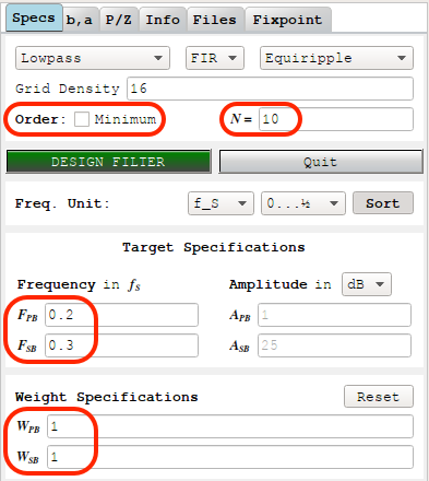
In pyFDA, we can calculate a half-band filter as follows:
-
Enter the pass band and stop band frequencies.
Make sure that the width of both bands are the same.
In the example above, the frequency range goes from 0 to 1/2, the pass band that ends at 0.2, and the stop band must start at 0.3 (= 0.5 - 0.2).
-
Deselect the “Order: Minimum” option.
As a result of this, we can now manually enter the order of the filter N, and the weights of the pass band and stop band Wpb and Wsb. We can not enter the attenuation parameters (Apb and Asb) any more.
-
Enter the desired filter order N
Choose a number that’s a multiple of 2, but not a multiple of 4.
Let’s use a value of 10, which corresponds to 11 coefficients.
-
Enter a value of 1 for both Wpb and Wsb, the ripple weigths for pass and stop band
If you didn’t change the default settings, you’ll see the following Magnitude Frequency Response graph after clicking “Design Filter”:
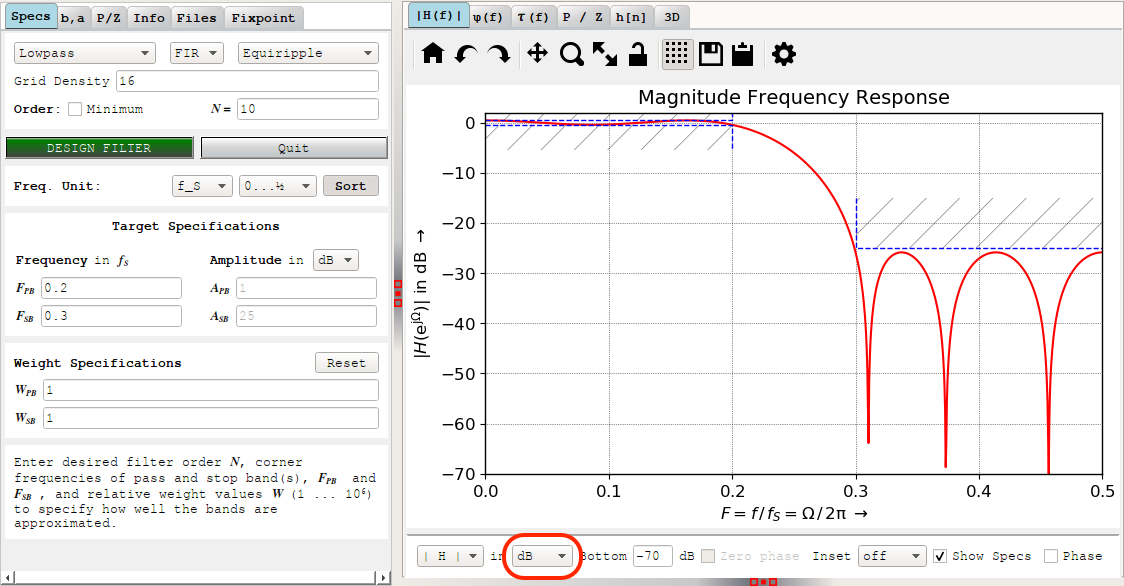
If you’re wondering why this doesn’t look symmetric at all, change the units from dB to V, you’ll be greeted with this:
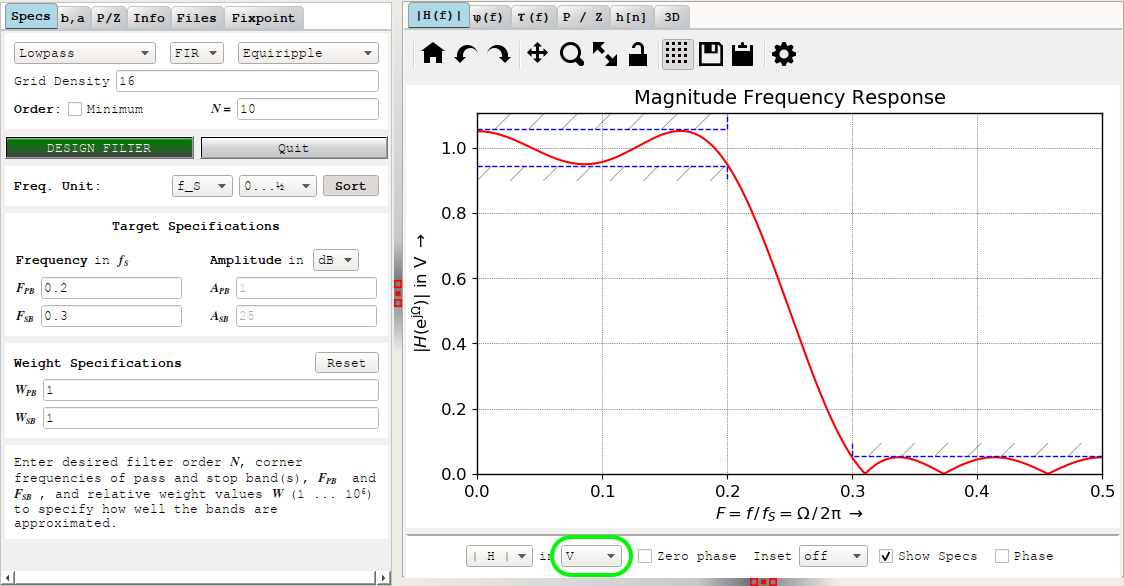
One again, the ripple in the pass band is identical to the ripple in the stop band, after taking into account that the negative ripple in the stop band comes out as positive because the magnitude response graph uses absolute values.
Click on h[n] tab in the right pane for the filter coefficients:
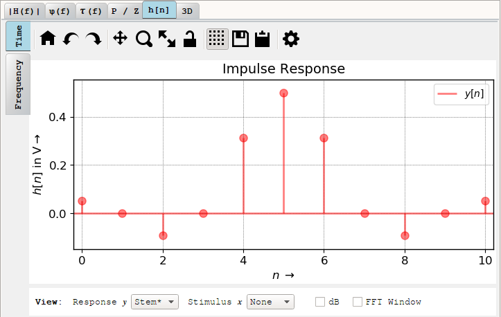
And, again, except for the center tap, 50% of the coefficients are 0.
Or are they? When you click select the b,a tab in the left pane, you get the coefficients
listed in floating point format:
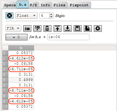
The coefficients are very close to but not quite 0. You can easily fix that by just clamping these coefficients to 0, but that doesn’t feel right, does it? For high order half-band filters with a high attenuation, this will almost certainly change the performance characteristics in some subtle way.
There must be a better way to go about this!
Designing Perfect-Zero Half-Band Filters with a Trick
Today, the Parks-McClellan/Remez algorithm to calculate FIR coefficients is fast enough even for very high order FIR filters. Even when implemented in Python.
This was definitely not that case in 1987. Back then, Vaidyanathan and Nguyen observed in A “Trick” for the Design of FIR Half-Band Filters that you can reduce the number of coefficients to calculate by (almost) 50% by transforming the half-band filter specification into a different FIR filter.
You’ll have to read the paper if you want to understand the details (it’s not super complicated), but the procedure is very simple.
Given a half-band filter specification with the following parameters:
- Filter order: N (and thus N+1 taps)
- N must be a multiple of 2 but not a multiple of 4
- Sample rate: Fs
- Pass band: from 0 to Fpb
- Stop band: from Fs/2-Fpb to Fs/2
Design a regular FIR filter with these parameters:
- Filter order: N/2
- Sample rate: Fs
- Pass band: from 0 to 2 x Fpb
- Stop band: from Fs/2 to Fs/2
The previous pyFDA example now has N halved from 10 to 5, Fpb doubled from 0.2 to 0.4, and Fsb is fixed at 0.5:
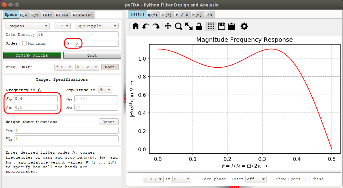
The stop band is gone now, but the pass band behavior of the magnitude frequence response graph has the same shape at the previous one.
And here are the coefficients:
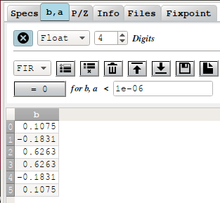
There are no zeros anymore, and values are exactly double of the non-zero coeffients of the values that were calculated without the trick! E.g. coefficient zero is 0.1075 vs 0.05372 earlier.
All that’s left now to get the half band filter coefficients is to divide the numbers above by half, insert a zero between each coefficient, except for the center coefficient which needs to be set to 0.5.
Half-Band Filter Design with NumPy
Just like generic FIR filters, I prefer a filter design script over a GUI. The code uses the trick and is straightforward:
def half_band_calc_filter(Fs, Fpb, N):
    assert Fpb < Fs/4, "A half-band filter requires that Fpb is smaller than Fs/4"
    assert N % 2 == 0, "Filter order N must be a multiple of 2"
    assert N % 4 != 0, "Filter order N must not be a multiple of 4"

    g = signal.remez(
            N//2+1,
            [0., 2*Fpb/Fs, .5, .5],         # The Trick
            [1, 0],
            [1, 1]
            )

    # Insert zeros
    h = [item for sublist in zip(g, zeros) for item in sublist][:-1]
    # Half coefficients
    h = np.array(h)/2
    # Set center tap
    h[N//2] = 0.5
To find the minimal filter order that satisfies both pass band and stop band attenuation, just increase the filter order until that condition is valid:
def half_band_find_optimal_N(Fs, Fpb, Apb, Asb, Nmin = 2, Nmax = 1000):
    for N in range(Nmin, Nmax, 4):
        print("Trying N=%d" % N)
        (h, w, H, Rpb, Rsb, Hpb_min, Hpb_max, Hsb_max) = half_band_calc_filter(Fs, Fpb, N)
        if -dB20(Rpb) <= Apb and -dB20(Rsb) >= Asb:
            return N

    return None
The code above is available on GitHub.
Using Half-Band Filters in Decimating Filters
With the design details out of the way, it’s time to understand why half-band filters are particularly useful for decimation filters.
Let’s first get out of the way that, even more than CIC filters, half-band filters are actually terrible when used stand-alone. This is because the attenuation of the filter at Fs/4 is by definition pegged 0.5 or -6dB. In a single stage 2x decimation filter, the stop band starts at Fs/4, so unless -6dB happens to be satisfactory for your design, a half band filter is out.
That’s why half-band filters are always used in multi-stage decimators.
Let’s show how that works with an example. In the figure below, I start out with an initial sample rate of 288kHz or a bandwidth of 144kHz, which I want to reduce to a sample rate of 48kHz, a factor 6x decimation. The signal of interest resides in the 0 to 10kHz spectrum, the pass band.

In a single stage implementation, I need an FIR filter with a pass band from 0 to 10kHz, and a stop band from 24kHz to 144kHz. The problem with that is that the transition band from 10kHz to 24kHz, 14kHz, is 1/10th of the overall bandwidth. Small ratios like this result in steep filters, and a large number of filter coefficients.

It’s better to split this filter into 2 stages: a 2x followed by a 3x decimation filter.
If we’d design the 2x decimation filter as if it were a single stage filter, we would put the end of the pass band at 24kHz, and put the start of the stop band to 72kHz. This ensures that the frequencies above 72kHz don’t alias into the remaining spectrum after decimation.

But that’s more than we need! In reality, we only need to make sure that the spectrum between 120kHz and 144kHz doesn’t alias onto the 0Hz to 24kHz. The part between 72kHz and 120kHz will alias to region between 24kHz and 72kHz, but we can remove that in the second filter.
What we end up with then is a passband from 0 to 24kHz and a stop band from 120kHz to 144kHz. Not only is this a very large transition band that requires far less filter coefficients, but we have symmetry: we can use a half-band filter and reduce the number of coefficients almost by half!
After the 2x decimation, we stil need the 3x decimation filter, but one that is half as steep as before, with the input sample rate half as well.

Let’s add a 0.1dB pass band and 90dB stop band requirement, and see how that works out in practice.
For a single stage 6x decimation filter, we’d end up with an FIR filter of order 80, resulting in:
48000 * 81 = 3,888,000 mul/s
Note how I’m multiplying the number of coefficients by the output sample rate of the filter, not the input sample rate!
Splitting things up in a 2x half band and a 3x FIR filter, we get a half-band filter of order 14, and an FIR filter of order 40:
Half band: 144000 * (14/2+1) = 1,152,000 muls/s
FIR:        48000 * 41       = 1,968,000 muls/s
Total:                         3,120,000 muls/s
In this case, the intermediate output sample rate of the half-band filter is 144kHz. The output sample rate of the final FIR filter remains at 48kHz.
We’ve reduced the number of multiplications by ~20%. That’s good, but it’s not spectacular. However, that’s because the overall decimation ratio is relatively small. We can see that the number of multiplication needs for the final FIR filter is almost 50% of what it used to be. Whether or not this 20% reduction is worth the complexity of having 2 stages vs just 1 will depend on the application.
For higher decimation ratios that contain multiple factors of 2, the following will happen:
- there will be more half-band stages, which will tilt the share of filtering work towards the more efficient half-band filters
- the steepness of the first half-band filter will be lower, which will reduce the number of coefficients for the first stage. Since that stage has the highest output sample rate, this effect will have a big impact on the number of multiplications.
In my previous blog post, I specified a PDM data rate of 2304kHz and an output PCM sample rate of 48kHz. I choose that ratio of 48 specifically because 48=3*16, which means that, if I want to, I can reduce the sample rate by a factor of 16 using nothing by half-band filters. (In practice, the initial decimation will be done by a CIC filter, which doesn’t require any multiplications at all, but that’s for later.)
Conclusion
Half-band filters are a tool to reduce the number of calculations in a multi-stage decimation filter. In this blog post, I focused on decimation filters only, but they are just as useful for interpolation filters.
I have now all the components that are necessary to design an efficient PDM to PCM processing pipeline. In the next installment, I’ll bring everything together and I’ll show a concrete implementation.
References
My Blog Posts in this Series
- An Intuitive Look at Moving Average and CIC Filters
- PDM Microphones and Sigma-Delta A/D Conversion
- Designing Generic FIR Filters with pyFDA and NumPy
- From Microphone Datasheet to Filter Design Specification
- Half-Band Filters, a Workhorse of Decimation Filters
- Design of a Multi-Stage PDM to PCM Decimation Pipeline
Filter Design
-
A ‘trick’ for the design of FIR half-band filters
Key paper that describes how to transform the parameters of a half-band filter to a different FIR filter with 1/2 of the filter taps, use the Remez algorithms to calculate those coefficents, and then use them for the half-band filter.
-
Halfband Filter Design with Python/SciPy
Simple example that shows how to calculate half-band filter coefficients with NumPy using the Remez algorithm and with a windowed sinc filter. However, it doesn’t use the trick.
-
Multiplier-Free Half-Band Filters
Excellent discussion about half band filters, ways to design them, and how to design them without multipliers. Also has an extensive example on how to convert from PDM to PCM with a CIC filter followed by 4 half band filters.
The website of this professor has a lot of course notes online. They are all worth reading.
Code
Decimation
-
Optimum FIR Digital Filter Implementations for Decimation, Interpolation, and Narrow-Band Filtering
Paper that discusses how to size cascaded filters to optimized for FIR filter complexity.