Designing Generic FIR Filters with pyFDA and NumPy
- Introduction
- Designing Filters with pyFDA
- Designing Filters with NumPy’s Remez Function
- Finding the Optimal Filter Order
- Complex FIR Filters
- Coming up
- References
Introduction
In my previous blog post, I promised that it was about time to start designing some real filters. Since infinite response (IIR) filters are a bit too complicated still, and sometimes not suitable for audio processing due to non-linear phase behavior, I implicitly meant finite impulse response filters. They are much easier to understand, and generally behave better, but they also require a lot more calculation power to obtain similar ripple and attenuation results than IIR filters.
There are many resources on the web that discuss the theoretical aspects about this or that filter, but fully worked out examples with full code are harder to find.
In this blog post, I will discuss the tools that I’ve been using to evaluate and design filters: pyFDA and NumPy.
I’ll almost always write ‘NumPy’ when discussing Python scripts related to this filter series. This should be considered a catch-all for various Python packages that aren’t necessarily part of NumPy: matplotlib for plots, SciPy for signal processing function, etc. I think it’s fair to do this because NumPy website lists SciPy as part of NumPy as well.
Matlab is popular in the signal processing world, but a license costs thousands of dollars, and even if it’s better than NumPy (I honestly have no idea), it’s total overkill for the beginner stuff that I want to do. GNU Octave is free software that’s claimed to be “drop-in compatible with many Matlab scripts”, but I haven’t tried it.
I’ve been told that a home license for Matlab is around 120 euros + 35 euros per toolbox. Cheaper than thousands, but still overkill.
Designing Filters with pyFDA
During initial filter configuration exploration, I often find it faster to play around with a GUI. It’s also a great way to learn about what’s out there and familiarize yourself with characteristics of different kinds of filters.
In a recent tweet, Matt Venn pointed me to pyFDA, short for Python Filter Design Analysis tool.
I’ve since been using it, and it definitely helped me in getting my PDM MEMS microphone design off the ground.
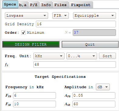
pyFDA’s GUI is split into 2 halves: parameters and settings on the left, results on the right.
In the parameters screenshot below I enter a low pass filter with pass band and stop band characteristics that we’ll later need for our microphone. I also ask it to come up with the minimum order that’s needed to meet these characteristics:
The default plot in the results section is the magnitude frequency response plot:
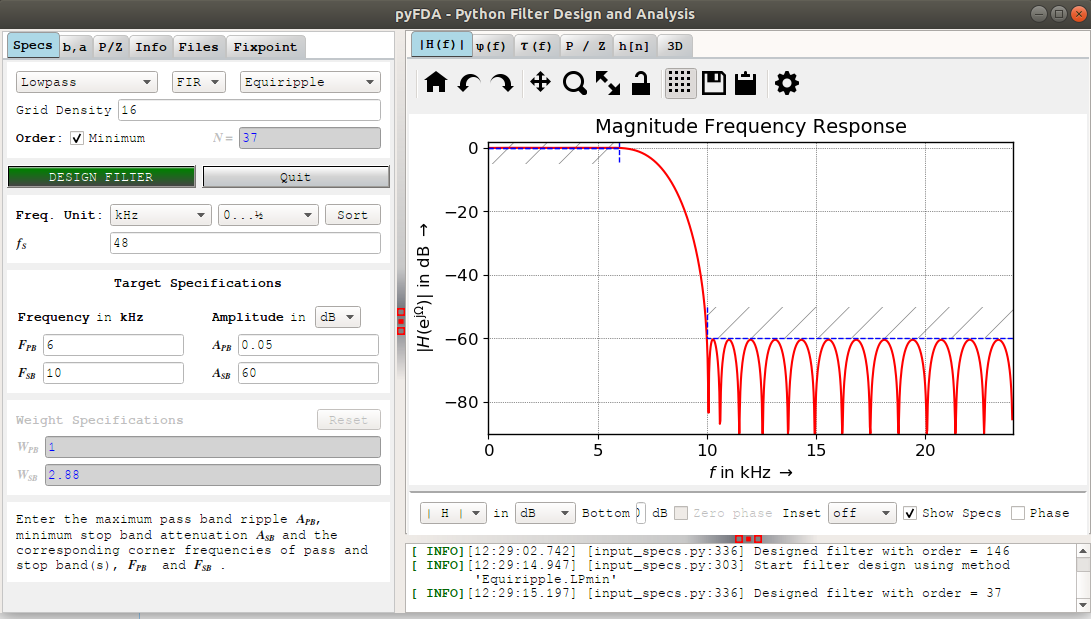
pyFDA tells us that we need a 37-order filter, which corresponds at 38 FIR filter taps.
There are all kinds of visualizations: magnitude frequency response, phase frequency response, impulse response, group delay, pole/zero plot, a fancy 3D plot that I don’t quite understand.
Once you’ve designed a filter, you can export the coefficients to use in your design, with or without conversion to fixed point numbers. pyFDA can even write out a Verilog file to put on your ASIC or FPGA.
Designing Filters with NumPy’s Remez Function
For all its initial benefits, once the basic architecture of a design has been determined, I prefer to code all the details as a stand-alone numpy file. For example, all the scripts that were used to create the graphs in this series can be found in my pdm GitHub repo.
Code has the following benefits over a GUI:
-
You can parameterize the input parameters and regenerate all the collaterals (coefficients, graphs, potentially even RTL code) in one go.
While writing these blog posts, I often make significant changes along the way. You really don’t want to manually regenerate all the graphs every time you do that!
-
Much more flexilibity wrt graphs
You can put multiple graphs in one figure, add annotations, tune colors etc. None of that is supported by the GUI.
-
It’s much easier for others to reproduce the results, and modify the code, learn from it.
Feel free to clone all my stuff and improve it!
The question is: how do you go about desiging FIR filters?
I’m not qualified to give a comprehensive overview, but here are some very common techniques to determine the coefficients of FIR filters. It’s probably not a coincidence that these techniques are also supported by pyFDA.
Moving Average and CIC Filters
I’ve already written about Moving Average and CIC filters. Their coefficients are all the same. pyFDA supports them by selecting the “Moving Average” option.
Windowed Sinc and Windowed FIR Filters
There are Windowed Sinc filters and Windowed FIR filters
where you specify a filter in the frequency domain, take an inverse FFT to get an impulse
response, and then use a windowing function to tune the behavior. NumPy supports these methods with the
firwin and
firwin2 functions.
Or use the “Windowed FIR” option in pyFDA.
While you can make excellent filters this way, they are often not optimal in terms of computational effort, and you need some understanding of the tradeoffs of this or that windowing filter to get what you want.
Equiripple FIR Filters
Finally, there are equiripple filters that are designed with the Parks-McClellan filter design algorithm. As far as I can tell, it is the most common way to design FIR filters and it’s what I used in my earlier pyFDA example by selecting the default “Equiripple” option.
It would lead too far to get into the details about the benefits of one kind of filter vs the other, but when given specific pass band and stop band parameters, equiripple filters require the lowest number of FIR coefficients to achieve the desired performance.
You can use the the remez
function in NumPy to design filters this way, and that exactly what I’ve been doing.
For example, the coefficients of the filter above in my pyFDA example, can be found as follows:
#! /usr/bin/env python3
from scipy import signal

Fs  = 48                # Sample rate
Fpb = 6                 # End of pass band
Fsb = 10                # Start of stop band
Apb = 0.05              # Max Pass band ripple in dB
Asb = 60                # Min stop band attenuation in dB
N   = 37                # Order of the filter (=number of taps-1)

# Remez weight calculation: https://www.dsprelated.com/showcode/209.php
err_pb = (1 - 10**(-Apb/20))/2      # /2 is not part of the article above, but makes the result consistent with pyFDA
err_sb = 10**(-Asb/20)

w_pb = 1/err_pb
w_sb = 1/err_sb

# Calculate that FIR coefficients
h = signal.remez(
      N+1,            # Desired number of taps
      [0., Fpb/Fs, Fsb/Fs, .5], # Filter inflection points
      [1,0],          # Desired gain for each of the bands: 1 in the pass band, 0 in the stop band
      [w_pb, w_sb]    # weights used to get the right ripple and attenuation
    )

print(h)
Run the code above, and you’ll get the following 38 filter coefficients:
[-2.50164675e-05 -1.74317423e-03 -2.54534101e-03 -7.63329067e-04
  3.77271590e-03  6.73718674e-03  2.64362264e-03 -7.87738320e-03
 -1.48337024e-02 -6.75502030e-03  1.48004646e-02  2.98724354e-02
  1.54099648e-02 -2.76986944e-02 -6.25133368e-02 -3.81892367e-02
  6.54474060e-02  2.09343906e-01  3.13554280e-01  3.13554280e-01
  2.09343906e-01  6.54474060e-02 -3.81892367e-02 -6.25133368e-02
 -2.76986944e-02  1.54099648e-02  2.98724354e-02  1.48004646e-02
 -6.75502030e-03 -1.48337024e-02 -7.87738320e-03  2.64362264e-03
  6.73718674e-03  3.77271590e-03 -7.63329067e-04 -2.54534101e-03
 -1.74317423e-03 -2.50164675e-05]
A little bit more additional code will create a magnitude frequency response plot:
import numpy as np
from matplotlib import pyplot as plt

# Calculate 20*log10(x) without printing an error when x=0
def dB20(array):
    with np.errstate(divide='ignore'):
        return 20 * np.log10(array)

(w,H) = signal.freqz(h)

# Find pass band ripple
Hpb_min = min(np.abs(H[0:int(Fpb/Fs*2 * len(H))]))
Hpb_max = max(np.abs(H[0:int(Fpb/Fs*2 * len(H))]))
Rpb = 1 - (Hpb_max - Hpb_min)

# Find stop band attenuation
Hsb_max = max(np.abs(H[int(Fsb/Fs*2 * len(H)+1):len(H)]))
Rsb = Hsb_max

print("Pass band ripple:      %fdB" % (-dB20(Rpb)))
print("Stop band attenuation: %fdB" % -dB20(Rsb))

plt.figure(figsize=(10,5))
plt.subplot(211)
plt.title("Impulse Response")
plt.stem(h)
plt.subplot(212)
plt.title("Frequency Reponse")
plt.grid(True)
plt.plot(w/np.pi/2*Fs,dB20(np.abs(H)), "r")
plt.plot([0, Fpb], [dB20(Hpb_max), dB20(Hpb_max)], "b--", linewidth=1.0)
plt.plot([0, Fpb], [dB20(Hpb_min), dB20(Hpb_min)], "b--", linewidth=1.0)
plt.plot([Fsb, Fs/2], [dB20(Hsb_max), dB20(Hsb_max)], "b--", linewidth=1.0)
plt.xlim(0, Fs/2)
plt.ylim(-90, 3)

plt.tight_layout()
plt.savefig("remez_example_filter.svg")
Run this and you get:
Pass band ripple:      0.047584dB
Stop band attenuation: 60.316990dB
And the following plot:

Check out remez_example.py
for the full source code.
Finding the Optimal Filter Order
In the example code above, the order of the filter (N=37) was given manually. To find the smallest N that satisfies the ripple and attenuation requirements, I just increase N until these requirements are met.
There are formulas to determine the filter order that’s needed to meet filter requirements, but they’re approximations. Useful 50 years ago when computing time was expensive, it made sense to use those, but that’s really not an issue today, so dumb brute force it is.
After factoring the earlier remez-based code as a function inside library
filter_lib.py,
it’s really as straightforward as this:
def fir_find_optimal_N(Fs, Fpb, Fsb, Apb, Asb, Nmin = 1, Nmax = 1000):
    for N in range(Nmin, Nmax):
        print("Trying N=%d" % N)
        (h, w, H, Rpb, Rsb, Hpb_min, Hpb_max, Hsb_max) = fir_calc_filter(Fs, Fpb, Fsb, Apb, Asb, N)
        if -dB20(Rpb) <= Apb and -dB20(Rsb) >= Asb:
            return N
Run the remez_example_find_n.py script:
from filter_lib import *

Fs      = 48000
Fpb     = 6000
Fsb     = 10000
Apb     = 0.05
Asb     = 60

N = fir_find_optimal_N(Fs, Fpb, Fsb, Apb, Asb)
And this is the result:
...
Trying N=33
Rpb: 0.086118dB
Rsb: 55.258914dB
Trying N=34
Rpb: 0.065989dB
Rsb: 57.550847dB
Trying N=35
Rpb: 0.048278dB
Rsb: 60.216487dB
Rpb: 0.048278dB
Rsb: 60.216487dB
Note that we need an FIR filter with order 35 (36 taps) to realize our requirements. In my example earlier, pyFDA with exactly the same parameters came up with a filter that’s 2 orders higher.
I have no idea why…
Complex FIR Filters
The remez function can handle much more than simple low pass, high pass, band pass or band stop filters.
You can specify pretty much any frequency magnitude behavior you want and make it come up with a set of FIR parameters.
I haven’t had a need for this yet. We’ll see if that changes in the future.
Coming up
In the next episode, I’ll have a look at the datasheet specifications of the microphone, and use that to determine the specification of our PDM to PCM design.
References
My Blog Posts in this Series
- An Intuitive Look at Moving Average and CIC Filters
- PDM Microphones and Sigma-Delta A/D Conversion
- Designing Generic FIR Filters with pyFDA and NumPy
- From Microphone Datasheet to Filter Design Specification
- Half-Band Filters, a Workhorse of Decimation Filters
- Design of a Multi-Stage PDM to PCM Decimation Pipeline
Filter Design
-
Remez (FIR design) Weights from Requirements
Shows how to calculate weights for the Remez algorithm (though there seems to be an off-by-2 error for the passband weights.)
-
Good presentation about different ways to design filters, Remez, ripple etc.
-
How to Create a Simple Low-Pass Filter
Simple explanation of how to do a windowed sinc filter. Numpy example code.
-
Online design tool for windowed sinc filters.