Polyphase Channelizers with Frequency Offset - a Bluetooth LE Example
- Introduction
- A Bluetooth LE Trace as Example
- Input Complex Heterodyne
- Derivation of Post-Decimation Offset Correction
- Simplifying for the Half-Bin Offset Case
- The Odd Case of an Odd Number of Channels
- Reducing the Number of Phase Adjustment Values
- Conclusion
- References
- Footnotes
Introduction
In previous blog post, I introduced the polyphase channelizer, a DSP algorithm that is incredibly efficient at heterodyning multiple channels to baseband in parallel. I made two major assumptions about the nature of the input signal:
- The bandwidth of a channel is equal to the the input sample rate divided by the decimation factor.
- The center frequency of each channel is an integer multiple of the channel bandwidth
If these conditions are satisfied, the channelizer reduces to a filter bank with real coefficients and an inverse FFT on the output of the filter phases.
In this blog post, I’ll use a real-world Bluetooth LE recording and a polyphase channelizer to extract all channels in parallel. There’s a twist, however, in that the center frequency of the channels is not a multiple of the channel bandwidth. With a little bit of additional math, we can work around that too.
I’m still roughly covering topics here that are covered in “Recent Interesting and Useful Enhancements of Polyphase Filter Banks” by fred harris, though my approach is more mathematical and less based on intuition. Furthermore, harris doesn’t work out the details for any generic frequency offset and immediately jumps to the half-channel case. But even there, he spends most of the time discussing a clever trick for odd decimation factors than the generic case that works for all decimation factors. I first deal with the full generic case and then simplify the outcome by imposing additional constraints.
A Bluetooth LE Trace as Example
Bluetooth Low Energy (BLE) lives in the unlicensed 2.4 GHz radio band that’s also used by wifi and many other protocols. It has 40 channels that are each 2 MHz wide for a total bandwidth of 80 MHz. The center frequency of the bottom physical channel is 2402 MHz. In total, BLE occupies a spectrum from 2401 MHz to 2481 MHz.
The 2.4 GHz radio band is often congested. To ensure that at least some packets get through, BLE uses frequency hopping: it continuously jumps from one channel to the next in some predictable pattern. However, to establish an initial connection, there are a number of fixed management channels.
Joshua used his BladeRF SDR unit to provide me with a 5 ms recording with the following characteristics:
- center frequency: 2.441 GHz
- sample rate: 96 MHz
- quadrature I/Q sampling
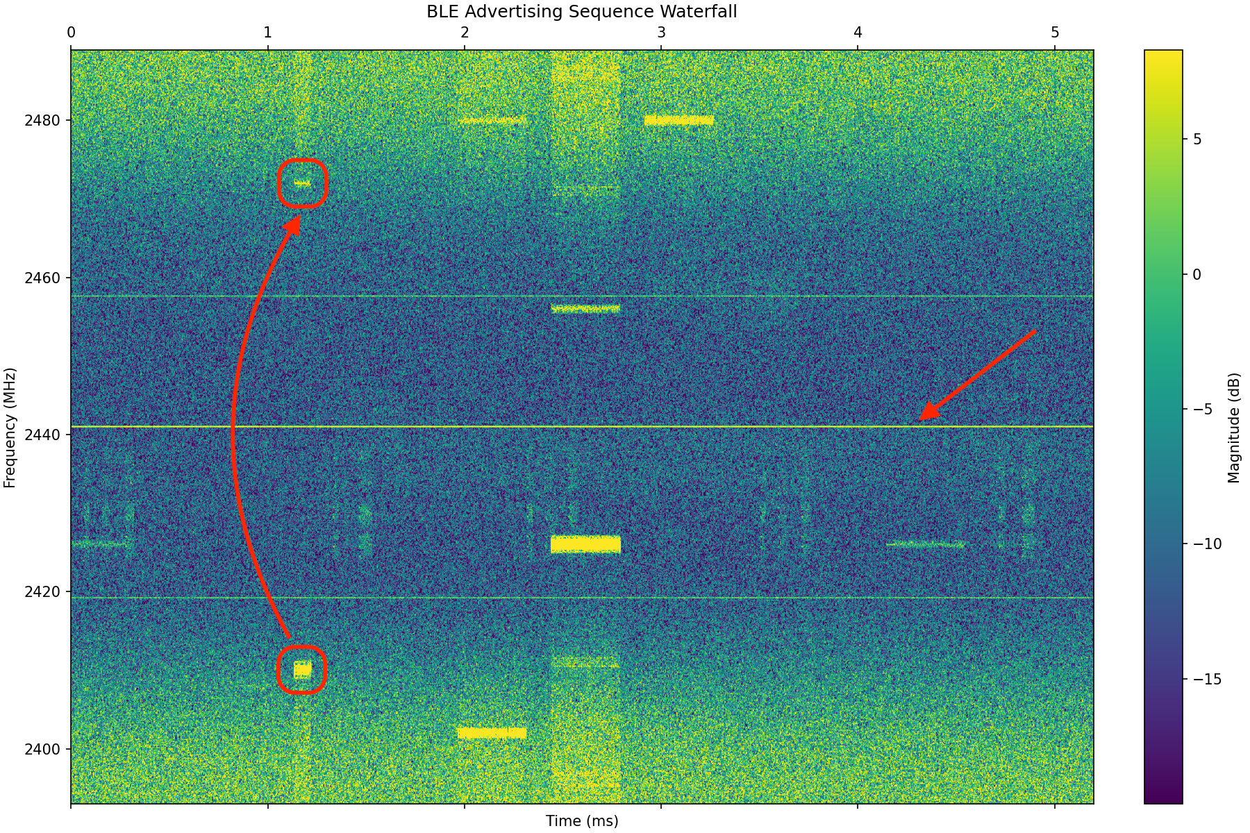
We can create a spectral power density waterfall plot of this, where the X-axis shows the time and the Y axis the short time Fourier transform (STFT) of the signal, showing the energy for the full frequency range.
 (Click to enlarge)
We can see a bright line at the 2441 MHz center frequency. This is a common artifact of the imperfect SDR hardware. It can be caused by local oscillator leakage or an imbalance between the I and Q channels of the quadrature AD converters, or both.
In his video, harris talks about how DC is often problematic, and a reason to have channels with a frequency offset so that none of the channel center frequencies coincide with DC. This trace shows why this is good advice.
We can also see some symmetry around the 2441 MHz line. For example, there’s a short burst around 1.1 ms at 2415 Mhz and a weaker version at 2467 MHz. This weaker version isn’t real either, but a spectral mirror image that’s caused by an imbalance between the I and the Q channels: their phase delta might not be exactly 90 degrees or they might have a slightly different gain on their way to the ADCs.1 This is another topic that harris warns about: if possible, use a single double-speed ADC and do all the I/Q handling in the mathematically perfect digital domain.
Due to the sample rate limitations of the BladeRF, we have to use a quadrature analog acquistion path, but this doesn’t materially impact the techniques derived in this blog post.
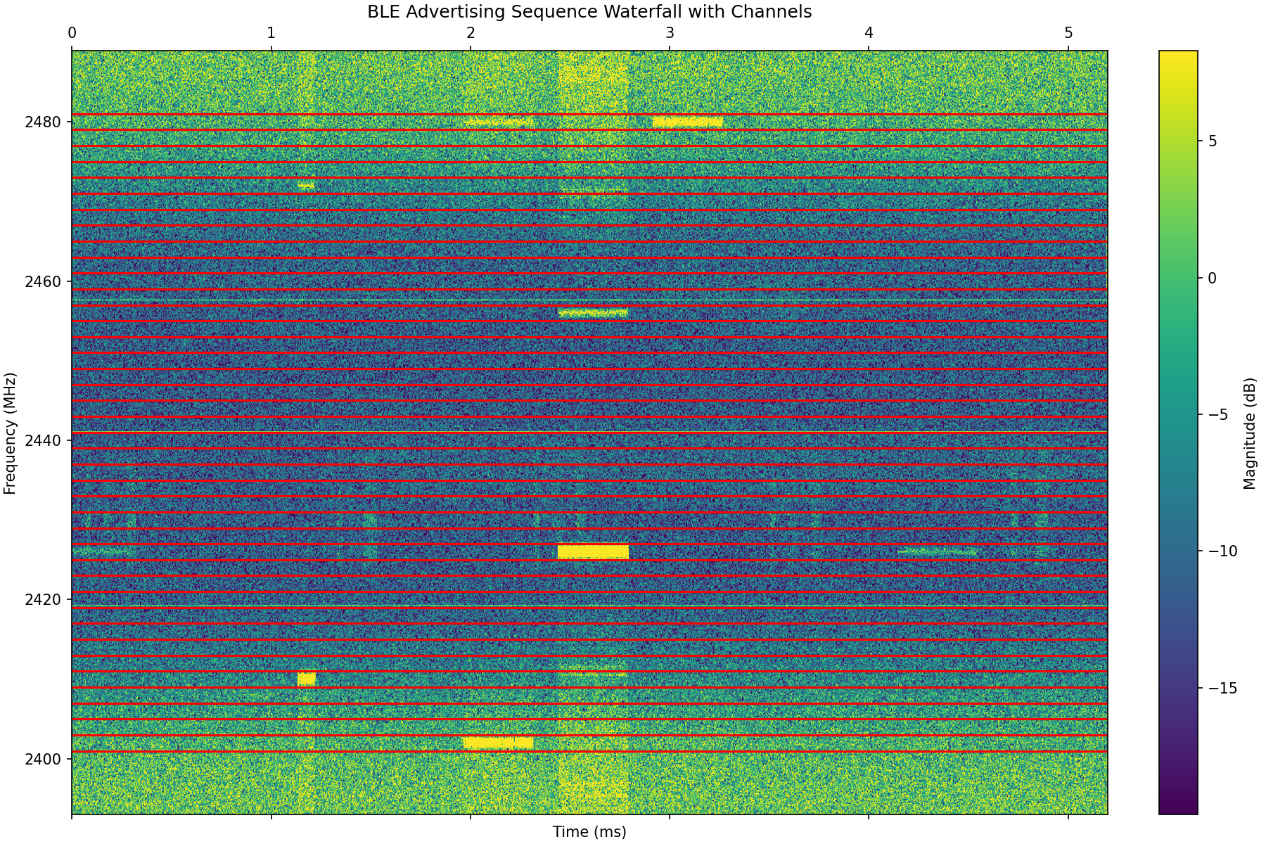
A recording of 96 Msps complex samples covers 48 channels of 2 MHz. Since BLE only has 40 active channels, we have a little bit too much data, but that’s ok. In the waterfall plot below, I’ve added separators between the individual channels. The suprious 2441 MHz line is now obstructed, which is good because it shows that it falls on a transition band.
 (Click to enlarge)
In the previous blog post, we operated under the assumption that channel center frequencies were located at a multiple of the decimated sample rate:
\[F_c = \frac{F_s}{M} c, \quad c = -\frac{M}{2}, \dots, -1, 0, 1, \dots, \frac{M}{2}-1\]
That’s not the case here. Instead, we have the following situation:
\[F_c = \frac{F_s}{M} c + \frac{F_s}{2M}, \quad c = -\frac{M}{2}, \dots, -1, 0, 1, \dots, \frac{M}{2}-1\]
Concretely, instead of channel center frequencies at -2, 0, 2, 4, … MHz, the BLE channels are located at -3, -1, 1, 3, 5, … MHz. Having the center frequency offset at exacty half the channel width is something we can exploit later, but I will first develop the generic case where the frequency offset can be anything, and then simplify.
Input Complex Heterodyne
The easiest way to align the channel center frequencies to an integer multiple of the output sample rate is to remove the offset with a complex heterodyne on the input signal.
Like this:
\[\omega_\Delta = 2 \pi \frac{F_\text{offset}}{F_s} \\ x[n] = x'[n] \, e^{j \omega_\Delta n} \\\]This works, but it undoes all the effort from last blog post where we tried very hard to not do any math at the input sample rate.
Still, let’s do it anyway and see what kind of result we get.
The code for the input heterodyne and the polyphase channelizer is below. I’ve stripped some of the comments for brevity, but check out the code in the GitHub repo for more details.
n = np.arange(len(ble_input), dtype=np.float32)

# Complex 1 MHz rotator to shift the spectrum by the half-channel offset
heterodyne_1mhz     = np.exp(1j * 2.0 * np.pi * channel_offset_hz / sample_rate_hz * n).astype(np.complex64)
# Do the heterodyne on the input signal
ble_input_pre_1mhz  = ble_input * heterodyne_1mhz

# Channel low-pass filter with a passband from 0 to 600 kHz
# and a stopband that starts at 800 kHz.
h_lpf = create_remez_lowpass_fir(
    input_sample_rate_hz     = sample_rate_hz,
    passband_hz              = 600e3,
    passband_ripple_db       = 1.0,
    stopband_hz              = 800e3,
    stopband_attenuation_db  = 50.0
    )

# Pad the filter with zeros so that the polyphase decomposition
# is a clean 2D array.
h_lpf   = np.pad(h_lpf, (0, -len(h_lpf) % decim_factor) )

# Polyphase filter decomposition:
# 48 rows, each row has interleaved coefficients.
h_lpf_poly  = np.reshape(
        h_lpf, ( (len(h_lpf) // decim_factor), decim_factor)
    ).T

# Polyphase decomposition/decimation of the input signal
ble_decim_pre_1mhz  = np.flipud(
    np.reshape(
        ble_input_pre_1mhz,
        ((len(ble_input_pre_1mhz) // decim_factor), decim_factor),
    ).T
)

# Calculate the output of all polyphase filters
h_poly_out_pre_1mhz = np.array(
        [np.convolve(ble_decim_pre_1mhz[_], h_lpf_poly[_]) for _ in range(decim_factor)])

# Vectorized IFFT to calculate the output of all channels
channel_data_pre_1mhz = np.fft.ifft(h_poly_out_pre_1mhz, axis=0).astype(np.complex64)
After extracting the data from channel 332 between 1.14 ms and 1.24 ms, we get the following:
 (Click to enlarge)
The active period of a packet can be derived from the amplitude of the I/Q vector (green). And the I/Q data clearly has some structure in it.
BLE uses Gaussian frequency shift keying (GFSK). Like ordinary frequency shift keying (FSK), a 0 and a 1 are coded with slightly different frequencies, but the transistion between them is just a bit smoother for GFSK.
Frequency is the derivative of the phase. Since I and Q are available, you can calculate the phase as follows3:
\[\phi[n] = \text{atan2}(q[n],i[n])\]The derivative is simply the delta between consecutive phase samples.
In Python, we can demodulate a GFSK signal like this:
angle = np.unwrap(np.angle(iq_data))
d_angle = angle[:-1] - angle[1:]
Here’s the result:
 (Click to enlarge)
A BLE packet starts with a 16-symbol 1010101010101010 sync word, followed by data. This definitely looks like a valid packet.
Cool! But it costs us a table with 48 rotator values that are fed into a complex multiplier, at the input sample rate. In this example, the input samples are already complex, but if they were real, the input heterodyne also forces all filter bank calculations to become complex.
Can we do better?
Derivation of Post-Decimation Offset Correction
Here’s the standard polyphase channelizer pipeline from last blog post:
 (Click to enlarge)
And here’s the mathematical description of the pipeline, for 3 channels and a filter with 9 coefficients:
\[\begin{alignedat}{0} y_c[n] & = & e^{j \frac{2 \pi}{3} c \, 0} & ( & h[0] & x[3n] & + & h[3] & x[3n-3] & + & h[6] & x[3n-6] & ) \\ & + & e^{j \frac{2 \pi}{3} c \, 1} & ( & h[1] & x[3n-1] & + & h[4] & x[3n-4] & + & h[7] & x[3n-7] & ) \\ & + & e^{j \frac{2 \pi}{3} c \, 2} & ( & h[2] & x[3n-2] & + & h[5] & x[3n-5] & + & h[8] & x[3n-8] & ) \\ \\ y_c[n+1] & = & e^{j \frac{2 \pi}{3} c \, 0} & ( & h[0] & x[3n+3] & + & h[3] & x[3n] & + & h[6] & x[3n-3] & ) \\ & + & e^{j \frac{2 \pi}{3} c \, 1} & ( & h[1] & x[3n+2] & + & h[4] & x[3n-1] & + & h[7] & x[3n-4] & ) \\ & + & e^{j \frac{2 \pi}{3} c \, 2} & ( & h[2] & x[3n+1] & + & h[5] & x[3n-2] & + & h[8] & x[3n-5] & ) \\ \end{alignedat}\]Let’s generalize this formula to \(M\) channels and \(N\) filter taps per phase:
\[y_c[n] = \sum_{m=0}^{M-1} \underbrace{ e^{j \frac{2 \pi}{M} c \, m} }_\text{IFFT} \sum_{k=0}^{N-1} h[kM + m] \; x[(n - k)M - m] \\\]Now substitute input \(x[n]\) with an input signal to which a complex heterodyne has been applied:
\[x[n] = x'[n] \; e^{j \omega_{\Delta} n}\] (Click to enlarge)
A frequency offset adjustment rotator has been introduced.
We can split up this exponential, extract a free-running output rotator that only depends on decimated sample number \(nM\), and move it all the way to the front:
\[y_c[n] = \underbrace{e^{j \omega_{\Delta} Mn} }_\text{output rotator} \sum_{m=0}^{M-1} e^{j \frac{2 \pi}{M} c \, m} \sum_{k=0}^{N-1} h[kM + m] \; x'[(n - k)M - m] \; e^{j \omega_{\Delta} (- kM - m)}\]Now extract the term that only depends on polyphase variable \(m\):
\[y_c[n] = e^{j \omega_{\Delta} Mn} \sum_{m=0}^{M-1} \underbrace{e^{-j \omega_{\Delta} m} }_\text{phase adjustment} e^{j \frac{2 \pi}{M} c \, m} \sum_{k=0}^{N-1} h[kM + m] \; x'[(n - k)M - m] \; e^{j \omega_{\Delta} (- kM)}\]Finally, rearrange the remaining exponential that is different for each filter coefficient index \(k\):
\[y_c[n] = \underbrace{e^{j \omega_{\Delta} Mn}}_{\text{output rotator}} \sum_{m=0}^{M-1} \underbrace{e^{-j \omega_{\Delta} m}}_{\text{phase adjustment}} \underbrace{e^{j \frac{2 \pi}{M} c \, m}}_{\text{IFFT}} \sum_{k=0}^{N-1} h[kM + m] \underbrace{e^{-j \omega_{\Delta} (kM)}}_{\text{filter adjustment}} \; x'[(n - k)M - m]\]There are 3 additional terms now:
- all the filter coefficients are modified by a filter adjustment term \(e^{-j \omega_{\Delta} (kM)}\).
- the output of each phase sub-filter is multiplied by a phase adjustment term \(e^{-j \omega_{\Delta} m}\).
- all outputs of the IFFT are subjected to complex heterodyne \(e^{j \omega_{\Delta} Mn}\).
None of this is ideal, but the first 2 terms are not dependent on the sample number and can be baked into the design. Meanwhile the rotator at the end not only runs at a rate that is M times lower, but the phase step of the rotator is also M times larger which reduces the size of a lookup table with rotator values.
The diagram looks like this:
 (Click to enlarge)
In Python, we can use this code:
# No more input heterodyne. Immediately decimate the input signal
ble_decim   = np.flipud(
    np.reshape(
        ble_input,
        ((len(ble_input) // decim_factor), decim_factor),
    ).T
)

# Calculate frequency offset
freq_offset           = channel_offset_hz / (sample_rate_hz / decim_factor)
omega_delta           = 2 * np.pi * freq_offset / decim_factor

# Modify the low pass filter coefficients
h_n                   = np.arange(len(h_lpf_poly[0]), dtype=np.float32)
h_lpf_poly_adj        = np.exp(-1j * omega_delta * decim_factor * h_n).astype(np.complex64)
h_lpf_poly_het        = h_lpf_poly * h_lpf_poly_adj

# Output of the polyphase filter
h_poly_out            = np.array([np.convolve(ble_decim[_], h_lpf_poly_het[_]) for _ in range(decim_factor)])

# Apply a phase rotation to the output of each phase
phase_nr              = np.arange(decim_factor, dtype=np.float32)
h_phase_adj           = np.exp(-1j * omega_delta * phase_nr).astype(np.complex64)
h_poly_out_phase_adj  = h_poly_out * h_phase_adj[:, None]

# IFFT...
channel_data          = np.fft.ifft(h_poly_out_phase_adj, axis=0).astype(np.complex64)

# Output rotator
sample_nr             = np.arange(channel_data.shape[1], dtype=np.float32)
heterodyne_1mhz_decim = np.exp(1j * omega_delta * decim_factor * sample_nr).astype(np.complex64)

# Heterodyne all channels
channel_data_1mhz_post  = channel_data * heterodyne_1mhz_decim[None, :]
While the channel I/Q output samples are not identical to the previous case due to a phase shift, the result after GFSK modulation is the same:
 (Click to enlarge)
This seems like a whole lot of effort for little benefit. Yes, we are running all operations at the output sample rate, but the number of multiplications per output sample is now higher than the case with the input heterodyne!
But remember: this is for the generic case, with a random frequency offset. Let’s fix that.
Simplifying for the Half-Bin Offset Case
As mentioned at the start of this blog post, it’s common to have a frequency offset that is equal to half the channel width:
\[F_\text{offset} = \frac{F_s}{2 M} \\ \omega_\Delta = 2 \pi \frac{F_\text{offset}}{F_s} = \frac{2 \pi}{2 M} = \frac{\pi}{M}\]A crucial observation is that 2 of our adjustment exponentionals feature a multiplication by \(M\).
The filter coefficients adjustment:
\[e^{-j \omega_\Delta (kM)} = e^{-j \frac{\pi}{M} (kM)} = e^{-j \pi k } = (-1)^k\]The output rotator:
\[e^{j \omega_\Delta (Mn)} = e^{j \frac{\pi}{M} (Mn)} = e^{j \pi n } = (-1)^n\]Awesome! The general equation has been simplified to this:
\[y_c[n] = (-1)^n \sum_{m=0}^{M-1} \underbrace{e^{-j \omega_{\Delta} m}}_{\text{phase adjustment}} \underbrace{e^{j \frac{2 \pi}{M} c \, m}}_{\text{IFFT}} \sum_{k=0}^{N-1} h[kM + m] (-1)^k \; x'[(n - k)M - m]\]The filter coefficients are real again and the complex multiplier for the output rotator can be replaced by logic that just inverts the sign of the output samples for each time tick.
 (Click to enlarge)
This is so much better! But it’s still possible to do better, though the requirements become even stricter.
The Odd Case of an Odd Number of Channels
We are currently still stuck with the per-phase complex rotator:
\[e^{-j \omega_\Delta m}\]When the channel center frequencies are offset by half the channel width, we’ve so far only considered an adjustment where the correction offset is half the channel bandwidth:
\[\omega_\Delta = \frac{\pi}{M}\]Relative to the full channel bandwidth of \(\frac{2 \pi}{M}\), this offset is \(r=0.5\).
\[\omega_\Delta = \frac{ 2 \pi }{M} r\]But \(r\) doesn’t have to be 0.5: we can use any kind of offset, as long as the fractional part of the value is 0.5.
For example, when \(r = 2.5\), the channelizer still works, but in addition to a fractional shift of half the channel width, there is an additional shift of 2 full channels. An output sample that would go to channel \(k\) for an offset of 0.5 now goes to channel \(k+2\) instead. Not the exactly the same result, but this reassigned output channel is just a minor bookkeeping issue.

Let’s see what happens when \(r=M/2\).
For even values of M, \(r\) is an integer value, without the fractional 0.5 half-bin offset that we need:

For odd values of M, we get the half-bin offset and all channels are moved by \(\frac{M-1}{2}\) at the output.

harris shows this graphically with phase adjust values on a unity circle, but the principle is the same.
Let’s see what \(r=M/2\) does to the phase adjust term:
\[r = M/2 \\ \omega_\Delta = \frac{ 2 \pi }{M} \frac{M}{2} \\ \omega_\Delta = \pi \\ e^{-j \omega_\Delta m} = e^{-j \pi m} = (-1)^m\]Nothing changes for the 2 other terms: for odd values of M, they still reduce to \((-1)^k\) and \((-1)^n\).
Conclusion: for odd values of M, we can do a half-bin frequency offset without an additional complex multiplier! Flipping the sign of some sub-filter output values and reassigning the output channel numbers is all that it takes.
 (Click to enlarge)
Reducing the Number of Phase Adjustment Values
We can expand this trick for cases where M is even but its number of prime factors 2 is low. Let’s do the exercise for \(M = 18\) and select \(r = \frac{M}{4} = \frac{18}{4} = 4.5\).
\[r = M/4 \\ \omega_\Delta = \frac{ 2 \pi }{M} \frac{M}{4} \\ \omega_\Delta = \frac{\pi}{2} \\ e^{-j \omega_\Delta m} = e^{-j \frac{\pi}{2} m} = 1, -j, -1, j, 1, \dots\]We didn’t get rid of the complex term, but we can implement these factors with a sign flip and/or swapping the real and imaginary part of the sub-filter outputs.
In general, if the following it true:
\[M = 2^p K, \quad K > 2\]Then you should choose \(r\) as follows:
\[r = \frac{M}{2^{p+1}} = \frac{K}{2}\]When \(p=0\), you get the case where M is odd, and adjustment factors of \({-1,1}\). When \(p=1\), the adjustment factors are \({-1,1, j, -j}\). For larger values of \(p\), you can’t avoid a complex multiplier, but at least you will limit the number adjustment values, which can be useful if you have 1 complex multiplier that serially processes all the sub-filter outputs before sending them to the IFFT.
For the BLE example:
\[M = 48 = 16 \cdot 3 = 2^4 \cdot 3 \\ r = \frac{48}{2^5} = 1.5\]With this configuration, the phase adjustment term wraps around at phase 32, so we only need a lookup table of 32 instead of 48 if we choose \(r=0.5\).4
Conclusion
Just like in previous blog post, we started with a straightforward solution to a problem that worked, but that required significant mathematical resources. We then threw some math at it and added constraints to simplify the math even more.
The outcome is once again appealing: for all decimation factors, the common case of shifting the spectrum by half the width of a channel requires at most one additional complex multiplication at the output of each sub-filter of the polyphase bank. And even this multiplication can be removed entirely if we can choose a decimation factor that is odd or if it only has one prime factor of 2.
All words in this blog post were written by a human.
References
-
Youtube - Recent Interesting and Useful Enhancements of Polyphase Filter Banks: fred harris
-
Analysis Channelizers with Even and Odd Indexed Bin Centers - fred harris
-
IEEE - Digital Receivers and Transmitters Using Polyphase Filter Banks for Wireless Communications
Other blog posts in this series
- Notes about Basic Polyphase Decimation Filters
- Complex Heterodynes Explained
- The Stunning Efficiency and Beauty of the Polyphase Channelizer
Source code
Footnotes
-
You can use Gram-Schmidt decorrelation to fix the I/Q vectors, supposedly, but I haven’t explored that yet. ↩
-
Channel zero is located at 2441 MHz. Channel numbers increment up to 24 the top frequency is reached, after which the frequency rolls over to the bottom and channel numbers continue to increment. That’s how you end up with 33. ↩
-
The \(\text{atan2}(q,i)\) function differs from \(\arctan(\frac{q}{i})\) function in the sense that the former works in all 4 quadrants whereas the latter only works in 1 quadrant. For DSP, you almost always need the 4 quadrant version. ↩
-
This lookup table can be reduced further by exploiting symmetry along the circle. ↩