Reed-Solomon Error Correcting Codes from the Bottom Up
- Introduction
- A Quick Recap on Polynomials
- Minimum Information to Define a Polynomial
- Some Often Used Terminology
- Reed Solomon Encoding through Polynomial Evaluation
- A Simple Error Correcting Reed Solomon Decoder
- A Systematic Reed-Solomon Code
- A Code Word as a Sequence of Polynomial Coefficients
- Polynomial Division in Hardware
- Reed-Solomon Encoding in Hardware
- Conclusion
- References
Introduction
I’ve always been intimidated by coding techniques: encryption and decryption, hashing operations, error correction codes, and even compression and decompression techniques. It’s not that I didn’t know what they do, but I often felt that I never quite understood the basics, let alone have an intuitive understanding of how they worked.
Reed-Solomon forward error correction (FEC) is one such coding method. Until the discovery of better coding techniques such as turbo and low-density parity check codes (LDPC), it was one of the most powerful ways to make data storage or data transmission resilient against corruption: the Voyager spacecrafts used Reed-Solomon coding to transmit images when it was between Saturn and Uranus, and CDs can recover from scratches that corrupt up to 4000 bits thanks to the clever use of not one but two Reed-Solomon codes.
The subject is covered in many college-level courses on coding and signal processing techniques, but a lot of the material online is theoretical, math heavy, and not intuitive. At least not for me…
That changed when I found this Introduction to Reed-Solomon article. It explains how polynomials and polynomial evaluation at certain points are a way to create a code with redundancy, and how to recover the original message back from it. The article is excellent, and it makes some of what I’m covering below unnecessary or redundant (ha!), because parts of what follows will be a recreation of that material. However my take on it has dumbed things down even more yet also covers a larger variety of Reed-Solomon codes.
One of the best aspects of that article is the focus on integer math. Academic literature about coding theory almost always starts with the theory of finite fields, also known as Galois fields, and then build on that when explaining coding algorithms. I found this one of the bigger obstacles in understanding the fundamentals of Reed-Solomon codes (and BCH codes, a close relative) because instead of getting to know one new topic, you now have to tackle two at the same time.
For this reason, everything in this blog post will use integer math as well. Integer math makes Reed-Solomon codes impractical for real world use, but it results in a better understanding about the fundamentals, before stepping up to the next level with the introduction of finite field math.
Many books are written about coding theory and applications, and a single blog post won’t even scratch the surface of the topic. I’m also still only beginning to understand some of the finer points. So my usual disclaimer applies:
I’m writing these blog posts primarily for myself, as a way to solidify what I’ve learned after reading stuff on the web. Major errors are possible, inaccuracies should be expected.
You’ll find some mathematical formulas below, but I always try to switch to real examples as soon as possible.
A Quick Recap on Polynomials
It’s impossible to discuss anything that’s related to coding without touching the subject of polynomials. You’ve probably learned about integer based polynomials during algebra classes in high school or in college but here’s a quick recap.
A polynomial \(f(x)\) of degree \(n\) is a function that looks like this:
\[f(x) = c_0 + c_1 x + c_2 x^2 + ... c_n x^n\]\(n+1\) fixed coefficients \(c_i\) are multiplied by function variable \(x\) to the power of \(i\) and added together. The polynomial can be evaluated by replacing variable \(x\) by some number for which you want to know the value of the function.
You can add, subtract, multiply or divide polynomials with each other.
Let’s illustrate this with some examples, and define \(f(x)\) and \(g(x)\) as follows:
\[\begin{aligned} f(x) & = 3 + 2 x + 5 x^2 - 4 x^3 \\ g(x) & = 7 x - x^2 \\ \end{aligned}\]Addition and subtraction work by adding or subtracting together the coefficients that belong to the same \(x^i\):
\[\begin{aligned} f(x)+g(x) & = (3+0) + (2+7) x + (5-1) x^2 + (-4+0) x^3 \\ & = 3 + 9 x + 4 x^2 - 4 x^3 \\ \end{aligned}\]You can multiply polynomials:
\[\begin{aligned} f(x) g(x) {} & = (3 + 2 x + 5 x^2 - 4 x^3)(7 x - x^2) \\ & = (3 + 2 x + 5 x^2 - 4 x^3)7 x + (3 + 2 x + 5 x^2 - 4 x^3) (-x^2) \\ & = 3 \cdot 7x + 2 x \cdot 7x + 5 x^2 \cdot 7x - 4 x^3 \cdot 7x + 3 \cdot -x^2 + 2 x \cdot -x^2 + 5 x^2 \cdot -x^2 - 4 x^3 \cdot -x^2 \\ & = 21 x + 14 x^2 + 35 x^3 - 28 x^4 - 3 x^2 - 2 x^3 - 5 x^4 + 4 x^5 \\ & = 21 x + 11 x^2 + 33 x^3 - 23 x^4 + 4 x^5 \\ \end{aligned}\]And you can divide them, using long division
\[\begin{aligned} \frac{f(x)}{g(x)} & = \frac{-4 x^3 + 5 x^2 +2x + 3}{-x^2+7x} \\ & = \begin{align*} &\text{ }\text{ }\text{ }\bf{4x+23}\\ -x^2 + 7x &\overline{\big)-4 x^3 + 5 x^2 +2x + 3}\\ &\underline{\text{ }-4 x^3 + 28 x^2}\\ &\text{ }\text{ }\text{ }-23x^2 +2x +3\\ &\text{ }\text{ }\underline{\text{ }-23x^2 + 161 x}\\ &\text{ }\text{ }\text{ }\text{ }\text{ }\text{ }\bf{-159x+3} \end{align*} \\ & = 4x+23 + \frac{-159x+3}{-x^2+7x} \\ \end{aligned}\]In the examples above, the coefficients \(c_i\), and function variable \(x\) are regular integers, but polynomials can be used for any mathematical system that has the concept of addition and multiplication.
Minimum Information to Define a Polynomial
Here’s one the most important characteristics of polynomials:
Any polynomial function of degree \(n-1\) is uniquely defined by any \(n\) points that lay on this function.
In other words, when I give you the value \(f(x) = c_0 + c_1 x + c_2 x^2 + c_3 x^3\) for any \(n\) distinct values of \(x\), you can derive the \(n\) coefficients \(c_0\) to \(c_{n-1}\), and these values \(c_i\) will be the same no matter which \(n\) values of \(x\) I used.
Here’s an example of a polynomial of degree 3, \(f(x)=2 + 3x -5x^2 + x^3\), evaluated for \(x\) values of \(-1,0,1,2\):
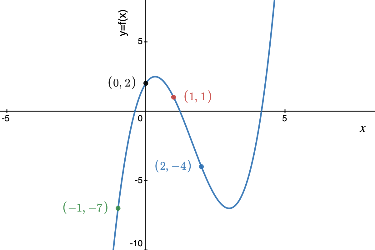
I used the excellent desmos graphing calculator to create this function plot.
When given the points \((-1, -7), (0,2), (1, 1), (2, -4)\), we can fill in the values into \(f(x) = c_0 + c_1 x + c_2 x^2 + c_3 x^3\) for each of point, which results in the following set of 4 linear equations with 4 unknowns:
\[c_0 + c_1 (-1)^1 + c_2 (-1)^2 + c_3 (-1)^3 = -7 \\ c_0 + c_1 (0)^1 + c_2 (0)^2 + c_3 (0)^3 = 2 \\ c_0 + c_1 (1)^1 + c_2 (1)^2 + c_3 (1)^3 = 1 \\ c_0 + c_1 (2)^1 + c_2 (2)^2 + c_3 (2)^3 = -4 \\\]This can be solved with the well-known Gaussian elimination algorithm. In our case, the values are such that we can solve it using a less systematic method:
The second row immediately reduces to \(\bf{c_0 = 2}\). When we fill that back in, the remaining rows become:
\[-c_1 + c_2 - c_3 = -9 \\ c_1 + c_2 + c_3 = -1 \\ 2 c_1 + 4 c_2 + 8 c_3 = -6 \\\]If we add the first and second row, we get: \(2c_2 = -10\), or \(\bf{c_2=-5}\), which simplifies the 3 rows to:
\[-c_1 - c_3 = -4 \\ c_1 + c_3 = 4 \\ 2 c_1 + 8 c_3 = 14 \\\]After substituting the second equation in the third one, we get:
\[2 c_1 + 8 (4 - c_1) = 14\]which reduces to \(-6 c_1 = -18\) or \(\bf{c_1 = 3}\).
And if we fill that into \(c_1 + c_3 = 4\), we get \(\bf{c_3 = -1}\).
Conclusion: \((c_0, c_1, c_2, c_3) = (2, 3, -5, 1)\). These coefficients match those of function \(f(x)\) that we started with!
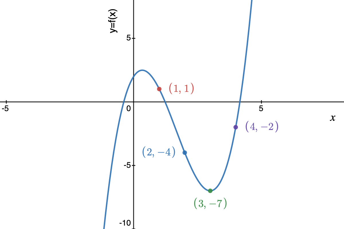
We can do the same exercise with points \((1, 1), (2, -4), (3, -7), (4, -2)\), and we’ll end up with the same result: \((c_0, c_1, c_2, c_3) = (2, 3, -5, 1)\). This is left as an exercise for the reader.
Note that Gaussian elimination isn’t the most efficient way to come up with \(f(x)\), since it requires a number of operations that is \(O(n^3)\). Construction of a Lagrange polynomial works just as well and that’s only a \(O(n^2)\) operations.
Some Often Used Terminology
There is no rigid standard about which kind of letters or symbols to use when discussing coding theory, but there’s a least some commonality between different texts.
-
a symbol
A symbol is the smallest piece of information. In many coding methods, a symbol is a single bit, with only two possible values. Reed-Solomon coding, however, uses symbols that have more than 2 values.
-
a message
A message is the original piece of information that need to be encoded. A message is a sequence of symbols.
For example, a message could be “Hello world “, where each character is a symbol.
-
a message word
A message word is a fixed length section of the overall message. Reed-Solomon coding is a block coding algorithm where a message is split up into multiple message words, and the encoding algorithm is performed on each message word without any dependency on previously received message words.
Message words are usually indicated with the letter \(m\), and \(k\) is often used to indicate the number of symbols in the message word. In other words, \(k\) is the size or the length of the message word.
In vector notation: \(m = (m_0, m_1, ... m_{k-1})\).
For example, if a message word is defined as having a size 4, our previous message would be split into the following message words: (‘H’, ‘e’, ‘l’, ‘l’), (‘o’, ‘ ‘, ‘w’, ‘o’), (‘r’, ‘l’, ‘d’, ‘ ‘).
-
an alphabet
An alphabet is the full set of values that can be assigned to a symbol.
\(q\) is often used as the number of values in an alphabet.
When a symbol is a single bit, the alphabet consists of 2 values, 0 and 1.
If we had a system where messages only consist of upper case and lower case letters and a space, then an alphabet could be (‘A’, …, ‘Z’, ‘a’, ‘b’, ‘c’, … , ‘z’, ‘ ‘), and the size of the alphabet would be 53. Almost all coding algorithms require the ability to perform mathematical operations such as addition, subtraction, multiplication and division on the symbols of a word, so don’t expect to see this kind of alphabet in the real world!
In practice, the alphabet of most coding algorithms is a sequence of binary digits. 8 bits is common, but it doesn’t have to be. I hesitate to call it an 8-bit number, because that would suggest that regular integer math can be used on it, and that’s almost never the case. Instead, the operations of such an alphabet use the rules of a Galois field.
-
a code word
A code word is what you get after you run a message word through an encoder. In the case of a Reed-Solomon encoder, a code word has a length \(n\) symbols, where \(n>k\) and the symbols are using the same alphabet as the message word.
Code words are often indicated with a vector \(s = (s_0, s_1, ... , s_{n-1})\).
When our message of three 4-symbol message words is converted into three 6-symbol code words, it could have the following code words:
(‘H’, ‘e’, ‘l’, ‘l’, ‘a’, ‘b’), (‘o’, ‘ ‘, ‘w’, ‘o’, ‘g’, ‘t’), (‘r’, ‘l’, ‘d’, ‘ ‘, ‘m’, ‘j’)
Notice how the first 4 symbols of each code word are the same as their corresponding message word, but that 2 symbols are added for error detection and correction. This makes it a systematic code. As we’ll soon see, not all coding schemes are systematic in nature, but it’s a nice property to have.
For Reed-Solomon codes, the length \(n\) of a code word must be smaller or equal than the number of values in the alphabet that it uses.
In all the examples below, the message words will have a length of 4, code words will have a length 6, and the symbols are using an alphabet of regular, unlimited range integers.
In other words: \(k=4\), \(n=6\), and the size \(q\) of the alphabet is infinite.
Using integers as symbols is a terrible choice: there are no real-world, practical Reed-Solomon implementations that use them. But as stated in the introduction, integer symbols allow us to focus on just the fundamentals of Reed-Solomon coding without getting distracted by the specifics of Galois field math.
If we’d want to send the “Hello world” message using an alphabet of integers, one possibility is to just convert each letter to their corresponding integer. For example, “Hello world “ would be converted to \((7, 30, 37, 37, 40, ...)\), because ‘A’ is assigned a value of 0, ‘B’ a value of 1, ‘a’ a value of 26, and so forth.
Reed Solomon Encoding through Polynomial Evaluation
Reed-Solomon codes were introduced to the world by Irving S. Reed and Gustave Solomon with a paper with the unassuming title “Polynomial Codes over Certain Finite Fields.” The 4-page paper can be purchased for the low price of $36.75. You should definitely not use Google to find one of the many copies for free.
Once you understand how Reed-Solomon coding and Galois fields work, the paper is quite readable, by today’s standards at least, and light on math too. Let’s get to business and explain how things work so that you can read the paper as well.
In an earlier section, we saw that we can set up a third degree polynomial with 4 numbers: either the 4 coefficients \((c_0, c_1, c_2, c_3)\), or 4 points \(f(x)\) on the polynomial for some given values of \(x\).
Once we know the coefficients, we can evaluate the polynomial at more than 4 values of \(x\). Those additional points are not required to specify the polynomial, they are redundant, which is exactly what we’re looking for: redundant information that allows us find the original values in case a code word gets corrupted during transmission!
And that’s what the original way of Reed-Solomon coding is all about:
Creating redundant information by evaluating a polynomial at more values of \(x\) than is strictly necessary.
Let’s go through a concrete example: I want to setup a communication protocol to transmit information that consists of a sequence of numbers, but I also want to add redundancy so that the message still can be recovered after a corruption.
Here’s one way to go about it:
Protocol Specification
The encoding and decoding parties must come up with some fixed parameters of the coding protocol that are not message dependent:
-
Agree on an alphabet.
-
Agree on the length \(k\) of the message word.
-
Agree on the length \(n\) of the code word.
The longer the difference in length between code word and message word, the more redundancy, and the more corrupted symbols can be error corrected.
-
Agree on how some polynomial \(p(x)\) should be constructed out of the symbols of the message word.
In the original paper the message word symbols are used as coefficients of this polynomial, but that’s not always the best choice. See later sections…
-
Agree on values of \(x\) for which to evaluate the polynomial \(p(x)\).
-
Agree that the code word is formed by evaluating \(p(x)\) at the numbers of \(x\) that were agreed on in the previous step.
That’s really it!
Let’s apply this to an example with the following protocol settings:
- The alphabet are integers.
- The size \(k\) of the message word \(m\) is 4.
- We want to 2 redundant symbols, so the code word has length \(n\) of 6.
- The polynomial \(p(x)\) is always evaluated for the following values of \(x\): \((-1, 0, 1, 2, 3, 4)\). Note that there are as many values \(x_i\) as there are symbols in a code word.
Here’s what happens to a message word with a value of \((2, 3, -5, 1)\):
Encoder
-
Create polynomial \(p(x)=2 + 3x -5x^2 + x^3\). It uses the message word symbols as coefficients.
I’m reusing here the polynomial that I used for the example in a previous section.
- Evaluate the polynomial \(p(x)\) at the 6 locations of \(x\): \((-1, 7), (0,2), (1, 1), (2, -4), (3, -7), (4, -2)\).
- The code word is: \((7,2,1,-4,-7,-2)\).
Decoder
Meanwhile, the decoder does the following:
- Get the 6 symbols of the code word. If there was no corruption, that’s still \((7,2,1,-4,-7,-2)\).
-
Take any 4 of the 6 received symbols, and link them to their corresponding \(x\) value.
If we take the first 4 code word symbols, we get \((-1, 7), (0,2), (1, 1), (2, -4)\).
-
Use these 4 points to derive the coefficients of the polynomial \(p(x)\) that was used by the transmitter.
We already saw how Gaussian elimination with the points \((-1, 7), (0,2), (1, 1), (2, -4)\) results in coefficients \((2, 3, -5, 1)\).
These coefficients are the symbols of the original message word!
The decoder picked 4 of the 6 code word symbols to recover the coefficients, and ignored the 2 others, so what was the point of sending those 2 extra symbols? A real decoder will be smarter and use those 2 additional symbols to either check the integrity of the received message, or to correct corrupted values.
A Simple Error Correcting Reed Solomon Decoder
Before decoding, let’s first talk about how many redundant symbols are needed to correct to correct errors:
To correct up to \(s\) symbol errors, you need at least \(2s\) redundant symbols.
In the example above, 2 additional symbols were added, which allows us to correct 1 corrupt symbol.
The original Reed-Solomon paper proposes the following algorithm:
- From \(n\) the received symbols of the code word, go through all combinations of \(k\) out of \(n\) symbols.
- For each such combination, calculate the coefficients of the polynomial.
- Count how many times each unique set of coefficients occurs.
- If there were \(s\) corruptions or less, the set of coefficients with the highest count will be coefficients of the polynomial that was used by the encoder.
Here’s how that works out for our example:
-
The decoder received the following code word: \((7, 2, 6, -4, -7, -2)\).
Notice how the third symbol isn’t 1 but 6. There was a corruption!
-
Associate each symbol with its corresponding \(x\) value: \((-1, 7), (0,2), (1, 6), (2, -4), (3, -7), (4, -2)\).
-
From these 6 coordinates, draw all combinations of 4 elements:
\[(-1, 7),(0, 2),(1, 6),(2, -4)\] \[(-1, 7),(0, 2),(1, 6),(3, -7)\] \[(-1, 7),(0, 2),(1, 6),(4, -2)\] \[(-1, 7),(0, 2),(2, -4),(3, -7)\] \[(-1, 7),(0, 2),(2, -4),(4, -2)\] \[(-1, 7),(0, 2),(3, -7),(4, -2)\] \[(-1, 7),(1, 6),(2, -4),(3, -7)\] \[(-1, 7),(1, 6),(2, -4),(4, -2)\] \[(-1, 7),(1, 6),(3, -7),(4, -2)\] \[(-1, 7),(2, -4),(3, -7),(4, -2)\] \[(0, 2),(1, 6),(2, -4),(3, -7)\] \[(0, 2),(1, 6),(2, -4),(4, -2)\] \[(0, 2),(1, 6),(3, -7),(4, -2)\] \[(0, 2),(2, -4),(3, -7),(4, -2)\] \[(1, 6),(2, -4),(3, -7),(4, -2)\]There are 15 combinations.
-
For each of these 15 combinations, determine the 4 polynomial coefficients:
\[(-1, 7),(0, 2),(1, 6),(2, -4) \rightarrow (2, 8, -5/2, -3/2)\] \[(-1, 7),(0, 2),(1, 6),(3, -7) \rightarrow (2, 27/4, -5/2, -1/4)\] \[(-1, 7),(0, 2),(1, 6),(4, -2) \rightarrow (2, 19/3, -5/2, 1/6)\] \[(-1, 7),(0, 2),(2, -4),(3, -7) \rightarrow (2, 3, -5, 1)\] \[(-1, 7),(0, 2),(2, -4),(4, -2) \rightarrow (2, 3, -5, 1)\] \[(-1, 7),(0, 2),(3, -7),(4, -2) \rightarrow (2, 3, -5, 1)\] \[(-1, 7),(1, 6),(2, -4),(3, -7) \rightarrow (19/2, 17/4, -10, 9/4)\] \[(-1, 7),(1, 6),(2, -4),(4, -2) \rightarrow (26/3, 14/3, -55/6, 11/6)\] \[(-1, 7),(1, 6),(3, -7),(4, -2) \rightarrow (7, 61/12, -15/2, 17/12)\] \[(-1, 7),(2, -4),(3, -7),(4, -2) \rightarrow (2, 3, -5, 1)\] \[(0, 2),(1, 6),(2, -4),(3, -7) \rightarrow (2, 18, -35/2, 7/2)\] \[(0, 2),(1, 6),(2, -4),(4, -2) \rightarrow (2, 49/3, -15, 8/3)\] \[(0, 2),(1, 6),(3, -7),(4, -2) \rightarrow (2, 13, -65/6, 11/6)\] \[(0, 2),(2, -4),(3, -7),(4, -2) \rightarrow (2, 3, -5, 1)\] \[(1, 6),(2, -4),(3, -7),(4, -2) \rightarrow (22, -56/3, 5/2, 1/6)\] -
The coefficients \((2,3,-5,1)\) come up 5 times. All other solutions are different from each other, so \((2,3,-5,1)\) is the winner. This is also the correct solution.
This may be a straightforward error correcting algorithm, but it’s not a usable one: even for this toy example with a message word of size 4 and only 2 additional redudant symbols, we need to determine the polynomial coefficients 15 times.
In the real world, a popular configuration is to have a message word with 223, and a code word with 255 symbols.
The formula to calculate the number of combinations is:
\[\frac{n!}{r!(n-r)!}\]With \(r=223\) and \(n=255\), this gives a total of 50,964,019,775,576,912,153,703,782,274,307,996,667,625 combinations!
That’s just not very practical…
It’s clear that a much better algorithm is required to make Reed-Solomon decoding useful. Luckily, these algorithms exist, and some of them aren’t even that complicated, but that’s worthy of a separate blog post.
A Systematic Reed-Solomon Code
Let’s recap how the previous encoder worked:
- The symbols of the message word are used as coefficients of a polynomial \(p(x)\).
- The polynomial \(p(x)\) is evaluated for \(n\) fixed values of \(x\).
- The code word is the \(n\) values of \(p(x)\).
This encoding system works fine, but note how all symbols of the code word are different from the symbols of the message word. In our example, message word \((2,3,-5,1)\) was encoded as \((7, 2, 6, -4, -7, -2)\).
Wouldn’t it be nice if we could encode our message word so that the original symbols are part of the code word, with some additional symbols tacked on for redunancy? In other words, encode \((2,3,-5,1)\) into something like \((2,3,-5,1,r_4, r_5)\). I already mentioned earlier that such a code is called a systematic code.
One of the benefits of a systematic code is that you don’t need to run a decoder at all if there is some way to show early on that the code word was received without any error.
It’s easy to modify the original encoding scheme into one that is systematic by treating the message word symbols as the result of evaluating a \(p(x)\) polynomial.
Encoder
- The message word symbols \((m_0, m_1, ..., m_{k-1})\) are the values of the polynomial \(p(x)\) at certain agreed upon values of \(x\).
- Determine the coefficients of this polynomial \(p(x)\) from the \((x_i, m_i)\) pairs.
- Evaluate polynomial \(p(x)\) for an additional \((n-k)\) values of \(x\) to create redundant symbols.
- The code word consists of the message word followed by the redundant symbols.
Let’s try this out with the same number sequence as before:
- The message word is still \((2,3,-5,1)\). These are now considered the result of evaluating polynomial \(p(x)\) for the corresponding values \((-1, 0, 1, 2)\) of \(x\).
-
Construct the polynomial \(p(x)\) out of these coordinate pairs: \(((-1, 2), (0, 3), (1, -5), (2, 1))\).
I found this website to do that for me. It uses the Lagrange interpolation method, but Gaussian elimination would have given the same polynomial.
The result is: \(p(x) = \frac{23}{6}x^3 + \frac{9}{2}x^2 + \frac{22}{3}x + 3\)
Note how some of the coefficients of \(p(x)\) are rational numbers instead of integers. This is one of the reasons why integers shouldn’t be used for Reed-Solomon coding!
- Evaluating \(p(x)\) for \(x\) values of 3 and 4 gives 44 and 147.
- The code word is \((2,3,-5,1,44,147).\)
The decoder is exactly the same as before!
A Code Word as a Sequence of Polynomial Coefficients
In the two encoding methods above, the code word consists of evaluated values of some polynomial \(p(x)\). There is yet another Reed-Solomon coding variant where the code word consists of the coefficients of a polynomial. And since this variant is the most popular, we have to cover it too. To understand how it works, there’s a bit more math involved, but an example later should make it all clear.
A message word has \(k\) symbols, and we need \(n\) symbols to form a code word. If a code word consists of coefficients of a polynomial, we need to create a polynomial \(s(x)\) of degree \((n-1)\).
Here are some desirable properties for \(s(x)\):
- \(k\) of its coefficients should be the same as the symbols of the message word to create a systematic code.
-
When \(s(x)\) is evaluated at \((n-k)\) values of \(x\), the result should be 0.
We’ll soon see why that’s useful.
Here’s a way to create a polynomial with these properties:
- Create a polynomial \(p(x)\) with symbols \((m_0, m_1, ..., m_{k-1})\) as coefficients, just like before.
-
Create a so-called generator polynomial \(g(x) = (x-x_0)(x-x_1)...(x-x_{n-k-1})\).
As before, the values \((x_0, x_1, ..., x_{n-k-1})\) are fixed parameters of the protocol and agreed upon between encoder and decoder up front. However, this time there are only are \((n-k)\) values of \(x_i\), as many as there are redundant symbols.
\(g(x)\) expands to \(g_0 + g_1 x + ... + g_{n-k}x^{n-k}\) and has a degree of \((n-k)\). Coefficient \(g_{n-k}\) will always be 1 due to the way \(g(x)\) is constructed.
-
Perform a polynomial division of \(\frac{p(x)x^{n-k}}{g(x)}\), such that \(p(x)x^{n-k} = q(x)g(x) + r(x)\).
In other words, \(q(x)\) is the quotient of the divison, and \(r(x)\) is the remainder.
- Define polynomial \(s(x)\) as \(p(x)x^{n-k} - r(x)\).
Let’s see what this gets us:
Desirable property 1: \(k\) coefficients of \(s(x)\) are \((m_0, m_1, ..., m_{k-1})\)
- \(p(x)\) has degree \((k-1)\). When multiplied by \(x^{n-k}\), that results in a polynomial \(m_{0}x^{n-k} + m_{1}x^{n-k+1} + ... + m_{k-1}x^{n-1}\). The degree of \(p(x)x^{n-k}\) is \((n-1)\), but its first non-zero coefficient is the one for \(x^{n-k}\).
- \(r(x)\) is the remainder of the division of polynomial \(p(x)x^{n-k}\), degree \((n-1)\), and \(g(x)\), degree \((n-k)\). The remainder of a polynomial division has a degree that is at most the degree of the divisor, \(g(x)\), minus 1: \((n-k-1)\). And thus, \(r(x) = r_0 + r_1 + ... + r_{n-k-1}\).
- There is no overlap in coefficients for \(x^i\) between \(p(x)x^{n-k}\) and \(r(x)\): \(r(x)\) goes from 0 to \((n-k-1)\) and \(p(x)x^{n-k}\) goes from \((n-k)\) to \((n-1)\). So if we subtract \(r(x)\) from \(p(x)x^{n-k}\), the coefficients of the 2 sides don’t interact. As a result, the coefficients of \(s(x)\) for terms \(x^{n-k}\) to \(x^{n-1}\) are the same as coefficients \(m_0..m_{k-1}\) of the message word. This satisfies the first desirable property.
Desirable property 2:\(s(x_i) = 0\)
- By definition, \(s(x) = p(x)x^{n-k} - r(x)\)
- By definition, \(p(x)x^{n-k} = q(x)g(x) + r(x)\), so after substitution: \(s(x) = q(x)g(x) + r(x) - r(x)\) and \(s(x) = q(x)g(x)\).
- By definition, \(g(x)= (x-x_0)(x-x_1)...(x-x_{n-k-1})\). Another substitution gives: \(s(x) = q(x)(x-x_0)(x-x_1)...(x-x_{n-k-1})\).
- \(x_i\) are roots of \(g(x)\), so fill in any value \(x_i\) and \(s(x_i)\) evaluates to 0!
What can we do with these properties? For that, we need to look at the decoder.
The decoder will use the code word symbols as coefficients of a polynomial \(s'(x)\). Without corruption, \(s'(x)\) is equal to \(s(x)\). Due to property 2, the decoder can verify this by filling in \(x_i\) into \(s'(x)\) and checking that the result is 0.
Each value \(s'(x_i)\) is called a syndrome of the received code word, so vector \((s'(x_0), s'(x_1), ..., s'(x_{n-k-1}))\) contains all the syndromes.
If a syndrome is not equal to 0, we know that the received polynomial \(s'(x)\) is not the same as the transmitted polynomial, and we can define an error polynomial \(e(x)\) so that \(s'(x) = s(x) + e(x)\). Polynomial \(e(x)\) has the same degree \((n-1)\) as \(s(x)\).
Since \(s(x_i) = 0\), it follows that \(e(x_i) = s'(x_i)\). There are \((n-k)\) values \(x_i\) and thus there are \((n-k)\) such equations. Expanded, the set of equations looks like this:
\[e_0 + e_1 x_0 + e_2 x_0^2 ... + e_{n-1} x_0^{n-1} = s_0 \\ e_0 + e_1 x_1 + e_2 x_1^2 ... + e_{n-1} x_1^{n-1} = s_1 \\ \cdots \\ e_0 + e_1 x_{n-k-1} + e_2 x_{n-k-1}^2 ... + e_{n-1} x_{n-k-1}^{n-1} = s_{n-k-1} \\\]If we can find a way to derive the \(n\) coefficients of \(e(x)\) out of the \((n-k)\) equations, we can derive \(s(x)\) as \(s'(x)-e(x)\). This is not generally possible: there are more unknowns than there are equations. But it is possible when the number of corrupted coefficients is half or less than \(n-k\), just like it was for the other coding variant.
A simple way to figure this out is again by going through all combinations and solving a set of equations.
Deriving an efficient general error correction procedure is complicated and outside of the scope of this blog post, but I’ll show a practical example where there’s only 1 corrupted but unknown symbol, just like the examples above.
Let’s once again start with message word \((2,3,-5,1)\) and go through the encoding and decoding steps.
Encoder
- The message word converts into polynomial \(p(x) = 2 + 3x - 5x^2 + x^3\).
- Let’s use \(x_0 = 1\) and \(x_1 = 2\) as roots of the generator polynomial: \(g(x) = (x-1)(x-2) = 2 -3x + x^2\).
- Divide \(p(x)x^2\) by \(g(x)\). WolframAlpha is perfect for this! It returns: \(x^5 - 5 x^4 + 3 x^3 + 2 x^2 = (x^3 - 2 x^2 - 5 x - 9)_{q(x)}(x^2 - 3 x + 2)_{g(x)} + (18 - 17 x)_{r(x)}\). We’re only interested in the last part, the remainder \(r(x) = (18 - 17 x)\).
- \(s(x) = p(x)x^2 - r(x)\) or \(s(x) = (2 x^2 + 3 x^3 -5 x^4 + x^5 ) - 18 + 17 x\).
- The code word is \((2, 3, -5, 1, -18, 17)\).
- As a verification step, you can fill in the values of 1 and 2 in \(s(x)\). They will evaluate to 0, as they should. Here is a way to do that with WolframAlpha…
Decoder
Let’s now do a decoding step when there’s was a corruption.
- The received code word is \((2, 3, -4, 1, -18, 17)\). The third symbol has been changed from -5 to -4.
- The received polynomial \(s'(x)\) is thus \(s'(x) = (2 x^2 + 3 x^3 -4 x^4 + x^5 ) - (18 - 17 x)\).
- Fill in the roots of \(g(x)\), 1 and 2, into \(s'(x)\) to find the 2 syndromes: \(s'(1)=1\) and \(s'(2)=16\).
- The syndromes are not 0, there was a corruption!
- There are 2 redundant symbols, so the maximum number of corrupted symbols we can recover is 1. The most straightforward way to figure out which symbol was corrupted is to go through all 6 possibilities and see if we get a consistent equation. Like this:
-
Let’s assume the first coefficient \(s_0\) is wrong, and all the others are right. In that case, \(s_0\) is an unknown, and all other coefficients are known: \(s(x) = s_0 x^2 + 3 x^3 -4 x^4 + x^5 - 18 + 17x\).
If we fill in \(x=1\), we get: \(s_0 +3 -4 +1 -18 +17 = 0 \rightarrow s_0 = -1\).
For \(x=2\): \(4 s_0 +24 -64 +32 -18 +34 = 0 \rightarrow s_0 = 1/2\).
We have contradicting values for \(s_0\), so we can conclude that \(s_0\) was not a corrupted coefficient.
-
We can do the same for all other coefficients. For all of them, you’ll get conflicting values, except for \(s_2\):
For \(x=1\): \(2 +3 + s_2 +1 -18 +17 = 0 \rightarrow s_2 = -5\).
For \(x=2\): \(8 +24 + 16 s_2 +32 -18 +34 = 0 \rightarrow s_2 = -5\). The values match!
- The received code word has been corrected to \((2, 3, -5, 1, -18, 17)\). The message word is the first 4 symbols of the code word.
Polynomial Division in Hardware
Reed-Solomon encoding with coefficients as code word is the method that you’ll most often find in the wild, and we just saw that it uses polynomial division.
How can we implement that in hardware?
Fundamentally, polynomial division works as follows:
- Start with the dividend as initial remainder.
-
Subtract a multiple of the divisor from the remainder so that its highest power of \(x\) becomes zero.
The multiple becomes a part of the quotient. What remains after the subtraction becomes the new remainder.
- Repeat the previous step until the highest non-zero coefficient of the remainder is for a power of \(x\) that is lower than the divisor.
This is exaclty what you do when performing a long division…
Here’s an example of dividing \((-2 x^7 + 3 x^5 - x^4 + 10 x^3 -4 x^2)/(x^3-3x^2+2x-1)\), performed in a spreadsheet:
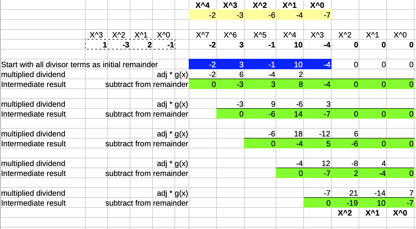
The quotient \(q(x)\) is \(-2 x^4 -3 x^3 -6 x^2 -4 x -7\) and the remainder \(r(x)\) is \(-19 x^2 + 10 x -7\).
Marked in blue is the initial remainder, which is identical to the dividend. Since the highest coefficient of the divisor is \(1\), the multiple by which the divisor gets adjusted is equal to the highest order coefficient of the remainder every step of the way.
However, the steps above require that the dividend is fully known at the start of the whole operation. In a real Reed-Solomon encoder, the dividend, \(p(x)x^{n-k}\) can have a lot of coefficients. For example, in the Voyager program, \(p(x)\) has 223 coefficients. It’d be great if we could rework the division so that we can perform it sequentially without the need to know the full dividend at the start.
We can easily do that:
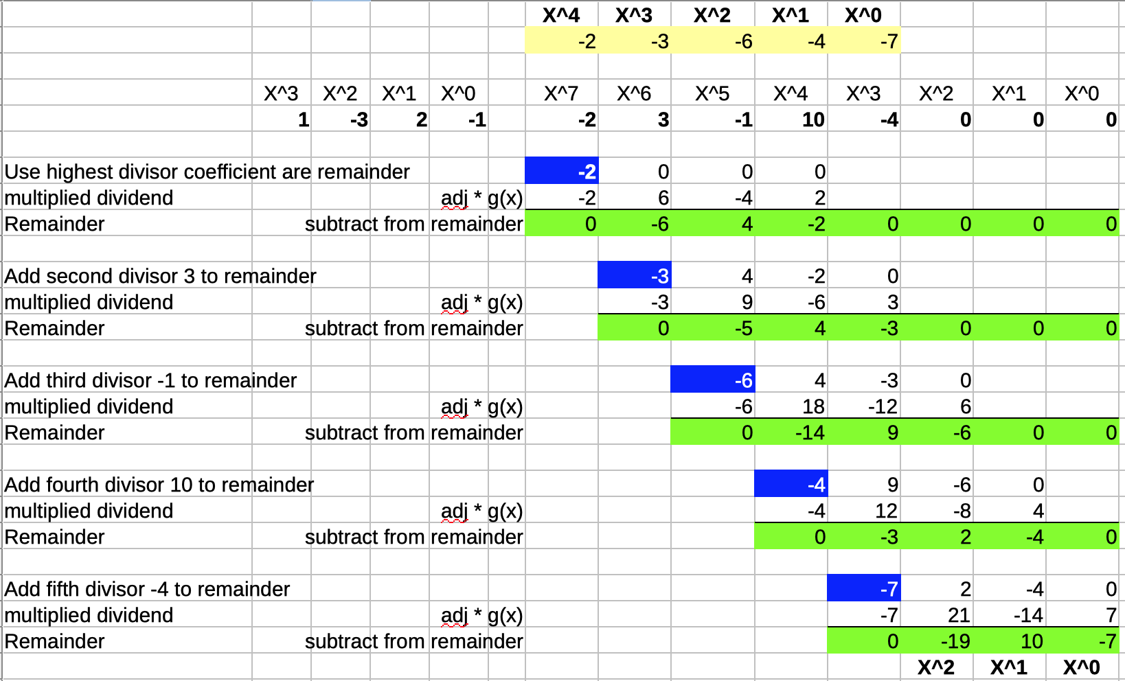
In the modified version above, instead of starting with a remainder that has all the terms of the dividend added to it, the coefficients of the dividend are added step by step, right when they’re needed to determine the next divisor multiplier. The result of the division is obviously still the same.
Also notice that the remainder, marked in green, has never more than 3 non-zero coefficients.
When performed sequentially, the divider above can be implemented with the following logic:
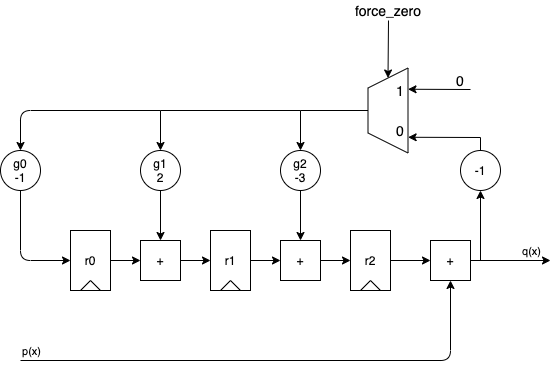
- At the bottom left, we have an input with the dividend \(p(x)\).
- On the right, there’s the output, which can either be the quotient \(q(x)\) or the remainder \(r(x)\),
dependent on whether
force_zerois deasserted or not. - 3 registers contain the current remainder
- The circles marked \(g_0, g_1, g_2\) multiply the divisor by the adjustment factor.
When we apply the dividend to the \(p(x)\) input in order of descending powers of \(x^i\), we get the following animation:
A full cycle is 8 steps:
- during the first 5 steps, the output contains the same quotient values as the one calculated by the long division.
- during the last 3 steps, the remainder rolls out.
- while shifting out the remainder values, the remainder registers are gradually re-initialized with a value of 0, so that a division operation can immediately restart again at step 1 for the next dividend.
Reed-Solomon Encoding in Hardware
In the previous section, we developed a sequential polynomial divider in hardware that outputs both the quotient and the remainder.
For a systematic Reed-Solomon encoder that outputs polynomial coefficients, the output should be the input, followed by the remainder. So a small modification is required:
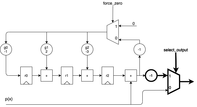
The only difference compared to the hardware of a regular polynomial divider is the addition
of an output multiplexer that allows us to route the input directly to the output.
force_zero and select_output can be wired together.
If you do a Google image search for “reed solomon encoder”, you’ll get a million variations of this diagram, with one exception: you won’t find any \(-1\) multiplier. This is because my Reed-Solomon encoder uses integer operations. In Galois math, subtraction and addition are the same operation.
The bus size of the hardware presented here is not defined, but for integer operations, the number of bits needed would be be much larger than the number of bits of the incoming symbols. That’s another big negative of using integers for these kind of coders. With Galois math, the result of any operation stays within the same range as the operands: an operation between 2 symbols that can be represented with 8 bits, will still be 8 bits, even if it’s a multiplication.
Conclusion
This concludes a first look at Reed-Solomon codes. There is a lot that was not discussed: Galois field mathematics, Galois field hardware logic, decoding algorithms, the link between Reed-Solomon codes and BCH codes, error corrections with erasures, and much more.
In the future, I’d love to try out Reed-Solomon codes on some practical examples, but who knows if I’ll ever get to that.
If you’ve made it this far, thanks for reading! I hope that this writedown was as useful for you as it was for myself.
References
-
Very good explanation on polynomial based interpolation and error correction.
Side story about Lagrange interpolation.
-
infectious - RS implementation
Code that goes with the RS article.
-
-
NASA - Tutorial on Reed-Solomon error correction coding (PDF file)
A very comprehensive but long tutorial that covers Galois fields, encoding, and decoding, with examples.
-
Relatively heavy on math, but one of the few articles that covers the different types of Reed-Solomon coding: the original method of encoding through polynomial values as well as the method of encoding polynomial coefficients.
-
Original paper: Polynomial Codes over Certain Finite Fields
Only 4 pages!
-
Voyager Telecommunications - Design and Performance Summary Series Article 4
Not very relevant, but an interesting overview of the telecommunications systems and the design considerations of the Voyager program.