Increasing Frequency Counter Precision with Linear Regression
- Introduction
- Frequency Counter Basics
- Calculating Frequency with a Linear Regression
- Some Caveats
- From Theory to Simulated Practice
- Digging Deeper
- References
- Footnotes
Introduction
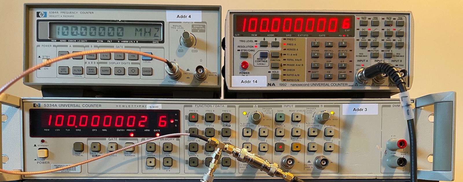
I don’t know how it happened, and it’s not that I’ve ever felt the need for more than one, but one way or the other I’ve ended up with 3 frequency counters in my collection of test equipment: first a Racal-Dana 1992, then an HP 5384A, and, recently, an HP 5334A. I’ve spent a good amount of time playing with them while testing oven controlled oscillators (OCXOs) and GPS modules.
 (Click to enlarge)
I also read up on the theory behind it. The basics are not super complicated, but to make sure I really understood some less intuitive aspects, I also ran some simulations to check that I really got things right.
One thing in particular was the concept of using linear regression to increase the accuracy of a frequency measurement.
This blog post first goes over some general frequency counter basics, it explains linear regression when applied to frequency counters, it shows linear regression in action with a Python simulation script, and it finishes with a lot of references related to time measurement.
Frequency Counter Basics
Most introduction texts on frequency counters start with the difference between conventional and reciprocal counters, so let’s get that quickly out of the way.
Conventional Counters
A conventional counter counts the number of input cycles over a fixed time period.
\[\text{frequency} = \frac{\text{input cycles}}{\text{measurement time}}\]If the time period is 1 second, then the value of the counter is the frequency of the input signal. Simple!
But it’s a terrible way of measuring the frequency of a signal, because the precision of the result depends on the frequency of the input signal: if the input signal is 10Hz and the measurement time is 1s, then the counter will capture 10±1 input edges, and that will be the measured frequency. For a 10MHz input signal, the counter will show 10,000,000±1.
The only way to increase the precision is to increase the measurement time.
Reciprocal Counters
In a reciprocal counter, there’s a second high-speed reference clock that is usually created by a reference oscillator. Cheap versions will have a regular crystal oscillators (XO), better ones a temperature controlled crystal oscillaotr (TCXO), and the best ones an oven controlled crystal oscillator (OCXO). The fixed reference frequency doesn’t matter a whole lot, but 10MHz is very common. Most frequency counters also have an external reference clock input for those who want their test equipment to be synchronized to a common clock, or when they want to use an ultra-stable reference clock such as a Rubidium clock reference or a GPS disciplined oscillator (GPSDO).
With an additional fixed-rate clock available, the frequency counter implements 2 counters: one that counts the edges on the input signal, like before, and one that counts reference clock cycles.
The measurement time from the earlier equation gets translated into a number of reference clock cycles:
\[\text{frequency} = \frac{\text{input cycles}}{\text{reference cycles} \cdot \text{reference clock period}}\]The frequency counter will still more or less measure over a desired time, say 1 second, but the measurement time isn’t exactly 1 second. Instead, counting starts and stops just before or just after an edge of the input signal.
The frequency calculation requires a division of two variables: the input signal counter, and the reference clock counter, hence the name reciprocal.
For example, if the input signal is ~10Hz, then a 10MHz reference cycle counter will start after an edge of the input counter. After ~1 second, the frequency counter will decide that it’s time to wrap things up. It will wait for an input edge, the 10th in this case, and stop the reference cycle counter. The input cycle counter will have a value of 10, the reference cycle counter a value of, say, 9,999,923.
The measured frequency will be:
\[\text{frequency} = \frac{10}{9,999,923 \cdot 10^{-7}s} = 10.00008 \text{Hz}\]The benefit of the reciprocal counter is clear: the result has a high precision even if the input signal has a very low frequency.
The waveforms below show how this works in practice:
 (Click to enlarge)
- A rising edge of the input signal resets the input counter to 0. It also starts a timer that determines how long we’d like to a measurement to last. This is the gate time.
- The first rising edge of the reference clock after opening the gate resets the reference counter.
- As long as the gate is open, every edge of the input signal and of the reference clock increments their respective counter.
- When the gate closes, the input counter stops counting immediately. The reference counter stops after the first edge that follows the input counter.
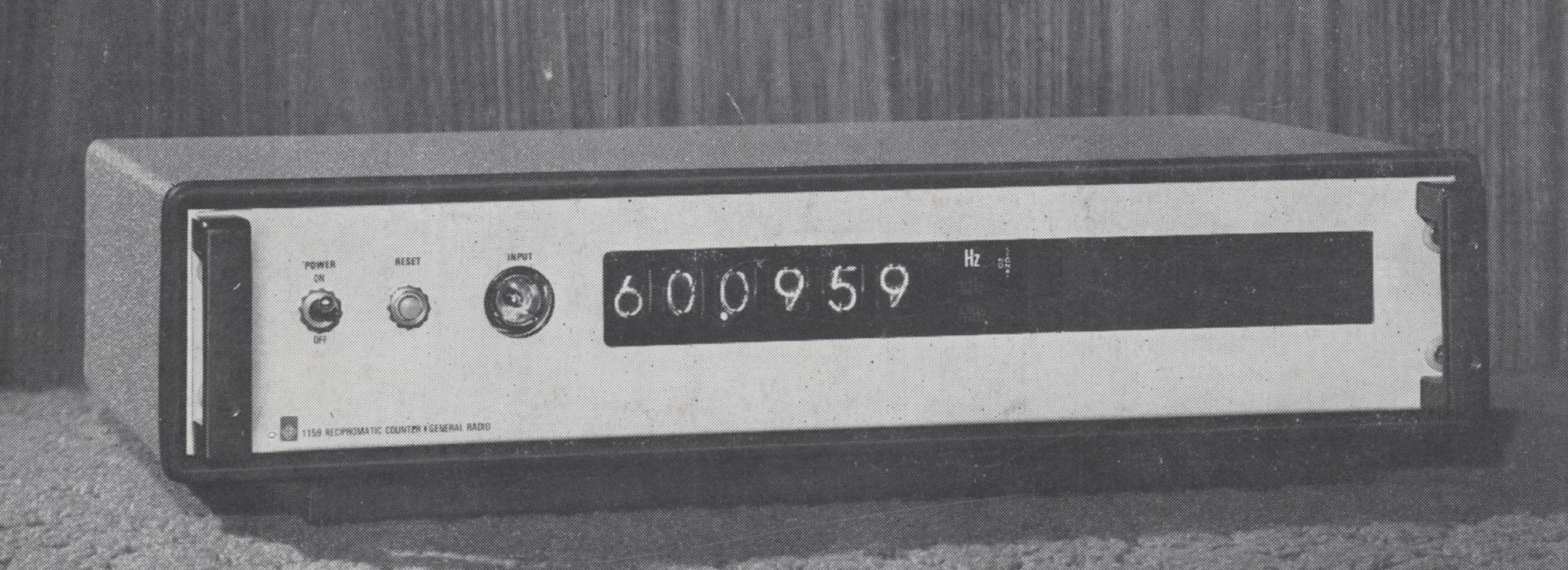
In the early days of electronics before microcontrollers, division by a variable number was an expensive operation, which is why these kind of counters came on the market later. But even then, there were already reciprocal counters on the market in the late 1960s, with the 6 digit General Radio 1159 Recipromatic Counter and the HP 5360A which used 500 TTL ICs to do the computation!
The waveform above shows where measurement errors are introduced in a reciprocal counter: the times indicated by the 2 arrows, \(T_{\text{start}}\) and \(T_{\text{stop}}\), between the first or the last edge of the input signal and the next edge of the reference clock, are not accounted for.
The two obvious ways to reduce those errors and increase the precision of a pure reciprocating counter are to increase the reference clock speed or to increase the gate time or both.
You can find quite a bit of very cheap DIY frequency counter projects on the Internet. Most of them are pure reciprocal counters. With a gate time of 1 second and a 10MHz reference clock, these counters have a theoretical precision of roughly 7 digits.
Interpolating Counters
10 seconds is about the practical measurement time limit, and it’s only in the past 25 years that running logic above 100MHz has become routine. Together, that will give you a precision of \(\log_{10}(10^8 \cdot 10)=9\) digits.
And yet, the aforementioned HP 5360A claimed a precision of 11 significant digits.
It does so by measuring \(T_{\text{start}}\) and \(T_{\text{stop}}\) in some other way and adjusting \(T_{\text{ref}}\) so that actual measured time is:
\[T_{\text{meas}} = T_{\text{start}} + T_{\text{ref}} - T_{\text{stop}}\]These kind of counters are called interpolating counters. Since we’re already at the digital clock speed limits, an interpolating counter uses alternative techniques to do the start-stop measurements. One way is to use a constant current to charge a capacitor during the start and the stop time and then measure the voltage across the capacitor with an AD converter, but there are other options too.
Interpolation can increase the resolution by a factor of 100 or more. Here’s the same picture with my counters again. All 3 are interpolating counters with a resolution of 9 digits1 when using a 1 second gate time.
In the setup above, the counters are not sharing the same reference clock and they haven’t been recently calibrated against a GPSDO, hence the lower digit difference.
The hybrid method of splitting up a time measurement into a coarse main measurement, and a start and stop fine measurement is called Nutt interpolation. The whole subject is worthy of a blog post by itself…
Improving accuracy and resolution by averaging
You can improve resolution by taking multiple measurements and averaging the results.
If we take \(n\) independent measurements, the accuracy improves by \(\frac{1}{\sqrt{n}}\). In other words, 100 measurements improve the accuracy by one digit.
Certain conditions must be true for this equation to be valid but the most important one is that the input frequency must be constant. That’s not always a given: despite being oven controlled, the frequency of an OCXO willl still vary a little bit when there’s a change in outside temperature, or even just due to drift. When you’re measuring with 12 digits of precision, those changes will be visible.
Also note that the formula holds for independent measurements, where the stop and start points of the previous and the current measurment are not the same. If you do multiple measurements where the stop of a previous measurement is the start of the next one, the accuracy actually improves by \(\frac{1}{n}\). Averaging 100 measurements improves the result by 2 digits.
However, that’s the essentially same as simply doing a single measurement that takes 100 times longer.
Still, averaging can be useful when you have frequency counter with only few gate time options. Older counters don’t support immediate restart, so the \(\frac{1}{\sqrt{n}}\) rule applies.
Continuous time stamping with linear regression
The final improvement is the subject of this blog post.
As before, we’re starting the input and reference counter after a certain edge of the incoming signal. And we’re stopping both counters after a certain gate time of, say, 1 second has expired.
But in addition to that, we’re also storing intermediate results, without stopping the counter. This is called continuous time stamping.
Each result is a pair \((x[k], y[k])\) that consists of a timestamp \(x[k]\) and an input counter value \(y[k]\).
After the gate time has expired, we’ll have a whole bunch of result pairs that will form a line when plotted on an (x,y) graph.
 (Click to enlarge)
There are different ways to process these pairs, but one of them is to a linear regression to find the best fitting line for the pairs. The ratio of that line is the measured frequency.
Calculating Frequency with a Linear Regression
Let’s take a step back and look at frequency counting as an (x,y) graph.
In the figure below, the horizontal axis is the reference clock counter and the vertical axis is the input clock counter.
 (Click to enlarge)
We can see that over 18 reference clock cycles, the input signal more or less toggles 7 times. “More or less”, because it doesn’t exactly toggle that much due to the \(T_{start}\) and \(T_{stop}\) errors from before.
At the bottom left, we see that the first input edge changes 62.5% into the phase of a reference clock cycle. And at the top right, the 7th input edge is rougly 25% into the phase of a reference clock cycle.
The frequency of the input signal is the ratio of the two signals divided by the reference clock period or multiplied by the reference clock frequency.
For a 10MHz clock, the exact calculation is
\[f = \frac{7}{17.25+0.375}\cdot 10^7 = 0.397163... \cdot 10^7 = 3.97163... MHz\]Since the counters are integer only for a non-interpolating counter, the coordinates that can be used for the calculation above must be rounded up or down for both end points. It doesn’t matter whether you round up or down, for different input values, you’ll get a better or worse result for either choice.
In the graph below, the green lines show the 2 worst choices: one line with the steepest and one with flattest slope. The real line is somewhere in between.
 (Click to enlarge)
The two extremes are
\[f = \frac{7}{17-0}\cdot 10^7 = 0.41176...\cdot 10^7 = 4.1176... MHz\]and
\[f = \frac{7}{18-(-1)}\cdot 10^7 = 0.36842...\cdot 10^7 = 3.6842... MHz\]So far, we’ve only sampled once. But what if we sample every 4 reference clock cycles? In the next graph we do exactly that. Every 4 clock cycles, we start looking for an input edge. The reference counter keeps running, but as soon as we see an input edge, we record both the value of the reference counter and the value of the input counter.
 (Click to enlarge)
The black dots are the true reference time stamps, but they are fractional. The green dots are the reference time stamps rounded down to the nearest integer.
You can see how the horizontal distance between two dots varies.
If we do a linear regression with all the samples, we’ll get a much better approximation of the input signal/reference clock ratio than with just one sample!
The LINEST() function in Excel and Google Sheets does that calculation for us:

The real ratio was 0.397163. Statistically, more samples will result in a better approximation of the real value. Note that in the example above, the result with only 3 samples is closer to the real value than the one with 5 samples. But as the number of samples goes up, the variance of result will go down.
Commercial frequency counters will use hundreds, thousands or more samples per measurement.
It should be clear that continuous time sampling with linear regression increases the precision of a frequency counter. Given enough samples, the increase in resolution is equal to:
\[\frac{2.45}{\sqrt{m}}\]where \(m\) is the number of samples.
Like the averaging case that was mentioned before, we can again see a \(\frac{1}{\sqrt{m}}\) factor here, but what we’ve gained is that the gate time for the full measurement hasn’t changed: we’ve added new measurements in the middle.
From there, you can derive the number of samples needed to increase the number of signficant digits by \(n\):
\[m = (2.45\cdot10^n)^2\]For example, to add 2 more digits, you need 60,025 samples.
The linear regression formula itself is:
\[f_{\text{input}} = \frac{m \sum{x_k y_k} - \sum{x_k}\sum{y_k}}{m \sum{x_k^2}-\sum{x_k}\sum{x_k}} \cdot f_{\text{ref}}\]A nice property of this formula is that you don’t need to retain the time stamping pairs: it’s sufficient to retain the running sums above in a couple of variables. At the end of the measurement, all you need to do are a few multiplications, subtractions, and a division.
    sum_xy = 0, sum_x = 0, sum_y = 0, sum_xx = 0;
    m = 0;

    while(!gate_time_expired){
        (x,y) = get_result_pair()
        sum_xy += x*y
        sum_x  += x
        sum_y  += y
        sum_xx += x*x
        m += 1
    }

    freq_input = (m*sum_xy - sum_x*sum_y) / (m*sum_xx-sum_x*sum_x) * freq_ref
Some Caveats
Linear regression works great… when it does, but that’s not always the case.
It requires a constant frequency throughout the whole measurement period. When the frequency changes a bit, maybe it’s a spread-spectrum oscillator, the linear regression will just fail and the result may not be better than the regular reciprocal method.
Linear regression also doesn’t help when you need to measure the time interval between two pulses. In that case, there’s really only two input edges: start and stop, and no way to extract multiple measurements.
But even when you want to measure a frequency, you won’t be able to extract a sufficient amount of samples if the input frequency is too low: you need 60,025 samples to gain two digits. When the input signal has a frequency of 1000Hz and the gate time is 1 second, then 1000 samples are the maximum of what you’ll be able to get.
From Theory to Simulated Practice
So much for the theory, let’s how these things translate into practice with a Python script that generates a bunch of timestamp pairs, and calculates the frequency with the traditional reciprocal method and with linear regression. The script that generates all the graphs below can be found here.
The inputs for each simulation are:
- the reference clock frequency
- the input signal frequency
- the total gate time or measurement duration
- the number of intermediate measurements or samples
Case 1: baseline example
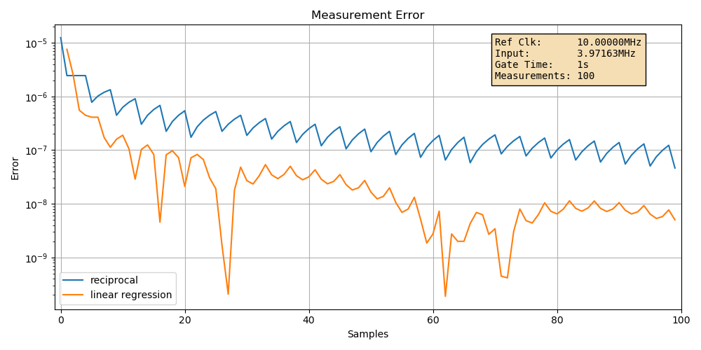
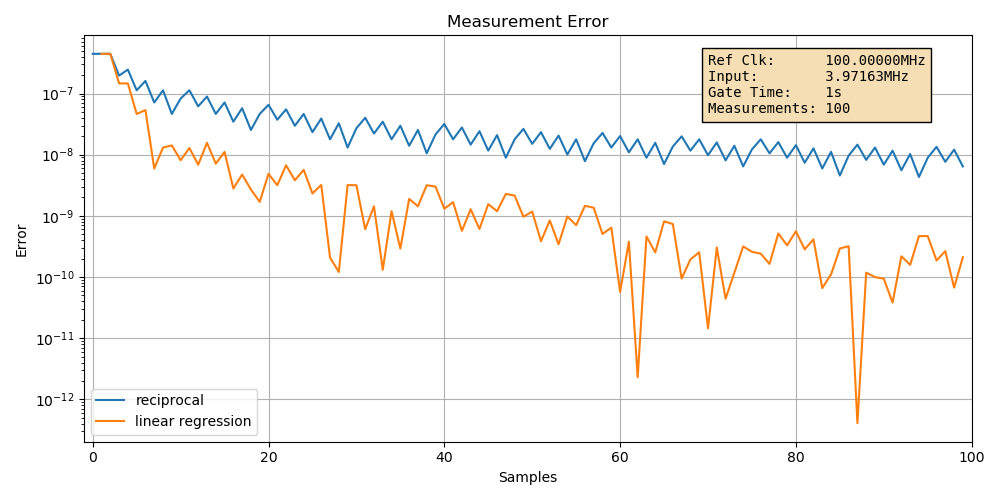
In the first graph, we’re looking at the input signal of the example above: a 10MHz reference clock, an input signal of 3.97163Mhz, a gate time of 1 second, and 100 measurements during that 1 second to do our linear regression.
 (Click to enlarge)
The graph shows the absolute relative error of the calculated frequency with a log scale, for an increasing number of samples.
Some basic observations:
-
there’s a general downtrend in the measurement errors.
There better be! The more data, the lower the error.
-
the errors are jittery.
This makes sense too. The variance of error goes down with increasing samples and duration, but it’s still a statistical distribution.
-
the error difference between the two methods is larger than expected.
Using the \(\frac{2.45}{\sqrt{m}}\) formula, you’d expect a difference of just 0.245 between the simple reciprocal and linear regression method, but we’re seeing an errors of roughly \(10^{-7}\) and \(5\cdot10^{-9}\) or a ratio of 0.005 instead.
That’s because the linear prediction error is an upper bound worst case.
The error of the simple reciprocal method is quite predictable: with a 1 second measurement duration and a 10MHz reference clock, you’d expect an error of around \(10^{-7}\). But the linear regresssion error is much harder to predict. We’ll get to that later.
Case 2: increasing the reference clock frequency to 100MHz
When we increase the reference clock frequency by a factor of 10, we should see the error of the reciprocal case go down by a factor of 10 as well, and that’s exactly what happens:
 (Click to enlarge)
The error has gone down from around \(10^{-7}\) to \(10^{-8}\). The linear regression error went down as well.
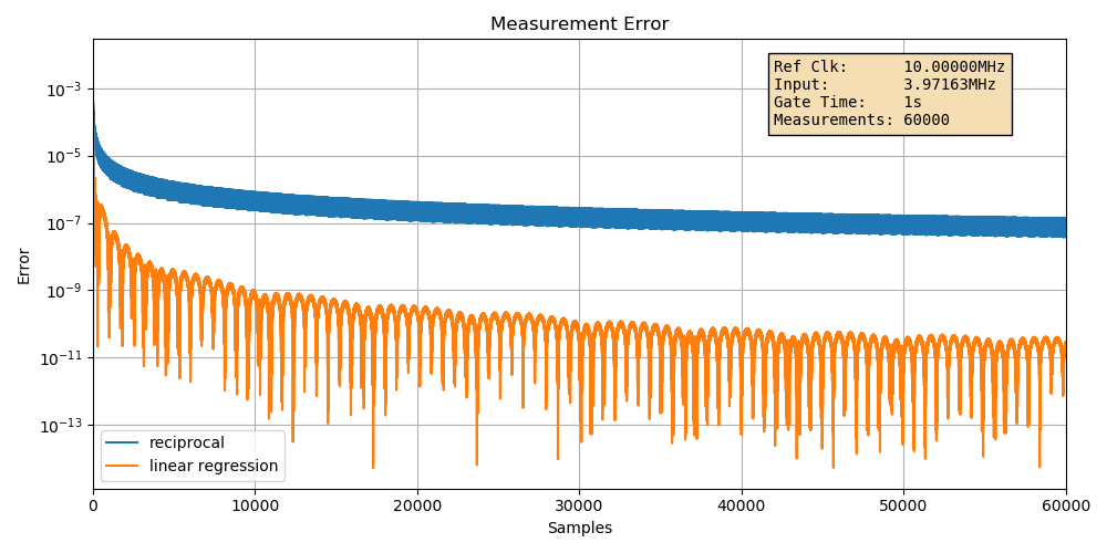
Case 3: baseline example with more intermediate sample points
Let’s go back to 10MHz, but increase the number of intermediate sample points from 100 to 60000.
 (Click to enlarge)
The reciprocal case only looks at the final end points, so at the far right of the graph we see the same error of around \(10^{-7}\) as for the baseline example.
Meanwhile, the error of the linear regression improves dramatically. The error is once again way lower than what’s predicted by the formula: we saw that we need 60,025 samples for an error difference of 2 digits. We’re seeing an error of around \(10^{-11}\), a difference of almost 4 digits!
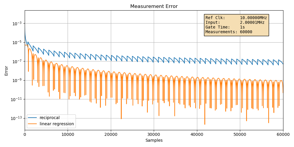
Case 4: worst case error example
So far, we’ve seen that the linear regression error reduction can be much better than the formula. I played around a bit with different input frequencies and found out that frequencies that are very close but not quite an exact integer factor slower than the reference clock tend to have the highest linear regression errors.
In this example, I’m using an input signal with a frequency of 2.00001MHz.
 (Click to enlarge)
While the input frequency is now different than before, the error for the reciprocal case is still the same: around \(10^{-7}\). Meanwhile, the linear error regression error is around \(10^{-9}\). That’s the worst case 2 digit difference in accuracy that you’d expect when using 60,000 samples!
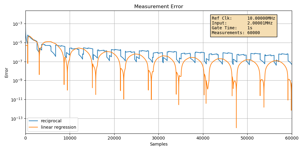
Case 5: unstable input signal
On of the key requirements for linear regression to work is that the input signal must be very stable.
Let’s what happens if we change the input frequency up and down by only one clock cycle back and forth:
 (Click to enlarge)
The error for both the reciprocal and the linear regression case are both worse, but more so for the linear regression case. The \(\frac{2.45}{\sqrt{m}}\) formula doesn’t hold anymore.
Digging Deeper
This blog post only scratches the surface of frequency measurements. There’s tons of information to be found the internet, some of it easy to understand, but most of it requires quite a bit of mathematical understanding.
In the references below, I’ve listed some of the material that I’ve used to write this blog post. There are also links to DIY frequency counter projects, forum discussions and more.
References
Linear regression frequency counting
-
Pendulum - New frequency counting principle improves resolution
Most of the content of this blog post is derived from this paper. Also contains detailed mathematical derivations without diving too deep into theory.
-
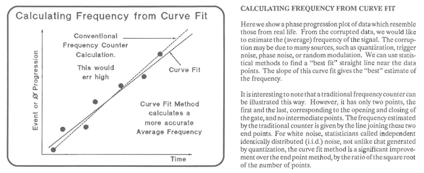
Analysis of Spread Spectrum Signals Using a Time & Frequency Analyzer
Presentation that’s not specifically about frequency counters, but it has the slide above that shows how curve fitting can be used to calculate frequency.
-
The Ω Counter, a Frequency Counter Based on the Linear Regression
Starts with short overview of different counters, then focuses on linear regression and how white noise is the main noise contributor in various elements of the system. Implements a counter in an FPGA and compares against other methods.
-
Discusses different weighing functions. Math heavy and way out of scope for this blog post.
-
Least-Square Fit, Omega Counters, and Quadratic Variance
Another mathematical derivation of the variance of different kinds of counters.
-
On the measurement of frequency and of its sample variance with high-resolution counters
Frequency counter basics
-
HP App Note 200 - Fundamentals of Electronic Counters
An excellent tutorial about various aspects of time measurements.
-
HP App Note 200-4 - Understanding Frequency Counter Specifications
Required reading if you want to better understand the specificiations of different frequency counters.
- Wikipedia - Simply Linear Regression
- NIST - Frequency and Time - Their Measurement and Characterization
- NIST - Handbook of Frequency Stability Analysis
DIY frequency counters
-
Low cost, high performance frequency/interval counters
DIY frequency counter with interpolation and linear regression.
-
A High Resolution Reciprocal Counter
Long blog post about building a DIY frequency counter.
-
EEVBlog: 8 – 11 digits reciprocal frequency counter 0.1 Hz – 150 MHz
Discussion about DIY frequency counter. Has multiple iterations of different designs, as well as info about linear regresssion. The whole thread is worth a read.
Commercial counters
None of the counters below have linear regression, but it’s still interesting to see how interpolating counters are built.
-
HP 5384A Operating and Service Manual
The theory of operation part in chapter 8 is excellent. It starts at section 8-151, page 8-21.
- HP 53131A Universal Counter Schematic
-
HP 53132A Universal Counter Schematic
The biggest difference between the two is that the 53132A has 2 interpolation ADCs, an 8-bit and a 10-bit one. The 53131A only has the 8-bit ADC.
Frequency counter history
- Antique Radios - Reciprocal Counters
- The General Radio Experimenter - The Recipromatic Counter
- HP Journal May 1969 - Introducing the Computing Counter
Random tidbits
-
A method for using a time interval counter to measure frequency stability
Not directly applicable, but interesting. Need to read more…
-
Simulation script for the graphs in the blog post.
Footnotes
-
The HP 5384A display shows only 8 digits, but its specification says it’s a 9 digit one. I should test this at some point by reading out values over GPIB. ↩